


 nueva página del texto (beta)
 Inglés (pdf)
 Artículo en XML
 Referencias del artículo
 Enviar artículo por email
 Citado por SciELO
  Similares en
SciELO
Similares en
SciELO 
 Permalink
1. INTRODUCTION
The L3 Lagrangian equilibrium point of the SunEarth system is a strategic point to observe the Sun. From there, it is possible to observe the opposite face of the Sun with respect to the Earth. Due to the rotation of the Sun, the observation of solar activity on the opposite side of the Sun could provide data to predict coronal mass ejections, of the order of weeks in advance. Predictions of this kind would be very important for many applications. Other types of observations could also be done from this point (Tantardini et al. 2010). Despite that, there are few researches exploring the Lagrangian point L3. Some reasons for this are the natural instability of the point for long duration missions, the perturbations from other planets and also the communication problem mentioned before, due to the location of the Sun, exactly between the Earth and the point L3. The instability exists for the point itself, as well as for orbits around this point. But it is important to remember that this type of instability also occurs for the other two collinear equilibrium points, L1 and L2. Despite this, many missions were planned for those two points (Gómez et al. 1993; Jorba & Masdemont 1999; Gómez et al. 1998; Koon et al. 2000; Llibre et al. 1985). Stable points are usually better places to locate spacecraft, but unstable points are also an option. In most cases, unstable equilibrium points are better places to locate a spacecraft, compared to a point with no equilibrium at all. Of course it is necessary to take care of the instability of the point, and an adequate stationkeeping strategy needs to be implemented to control this natural instability, as well as other perturbations from other forces (Tantardini et al. 2010). For these reasons, previous researches considered orbits near those points (Barrabés & Ollé 2006), and even transfer orbits to those points (Prado & Broucke 1995; Hou, X., Tang, J., & Liu, L. 2007). The perturbations from other planets, in particular Venus, may be reduced using an adequate choice for the date for the mission (if it is not too long) or by using control techniques.
The present research aims to find some simple alternatives to solve the communication problem for a satellite equipped with a solar sail by shifting the location of the equilibrium point from the Ecliptic plane. Solutions are found in the plane perpendicular to the Ecliptic plane of the Sun-Earth system which contains the collinear Lagrangeanpoints. This is done by considering not only the Earth and the Sun gravitational interactions with the satellite, but also the force due to solar radiation pressure. With this more complete model, new equilibrium points appear, with locations different from the ones obtained considering only gravitational forces. Thus, a proper choice of the parameters of the solar sail, like its size, attitude, reflectance properties, etc., can achieve a location of the point away from the orbital plane of the Earth. This out-of-plane component can shift the point to ensure direct visibility from the point to the Earth. This idea could also be used to make measurements related to relativity theory, by verifying the distortion of the light passing near the border of the solar disk. Basically, new “artificial equilibrium points” appear, which are points where the resultant of the accelerations is zero in the noninertial frame of reference. They are new points, because they are obtained with the inclusion of the non-gravitational force given by the solar sail. This concept was already used to study the possibility of placing a mirror around the Earth to either increase the temperature of our planet (Salazar et al. 2016), or to decrease it (McInnes 2010). Other references using this concept in different equilibrium points are given by Morimoto et al. (2007) and McInnes et al. (1994). Research in attitude and trajectory stability of solar sails was done by Li (2015). One alternative is to place a second satellite, also equipped with a so lar sail, at a new artificial equilibrium point near L1. Another alternative is to place a spacecraft “below” the traditional equilibrium point L3 on the ecliptic plane. Out-of-plane displacements of these points can also help the link between the satellite near L3 and the Earth, as we show in detail later. Thus, three strategies are proposed to remove the problem of visibility between L3 and the Earth, helping to make this particular point available for astronautical applications.
2. MATHEMATICAL MODELS
According to the Coriolis theorem (Symon 1986), the equation of motion of a spacecraft under the gravitational influence of the Sun and the Earth and subjected to a force due to the solar radiation pressure over its sail, written in a non-inertial rotating frame of reference that has the Sun fixed at its center is given by:
where:
The rotating frame of reference is shown in Figure 1, where the bodies involved (Sun, Earth and spacecraft) and the new artificial equilibrium point near L3 can be seen. The Sun is placed at the center of the reference system, with the Earth in a circular orbit at radius R. The satellite equipped with a solar sail - a flat one - remains fixed in the artificial equilibrium point near L3. In particular, the out-ofplane component of its location is noted, marked by he. In order to obtain this equilibrium, the vector normal to the solar sail has to make an angle γe with the direction of the solar rays. In this geometry, the line Sun-spacecraft makes an angle α with the orbital plane of the Earth. The force due to the solar radiation pressure on a flat solar sail with perfect reflection is given by McInnes (2004) as:

where R is a positive constant that represents the Sun-Earth distance, pe
is the solar radiation pressure at a distance R from the Sun, A is the total area of
the sail,
For the purpose of this study, the motion of the Earth around the Sun is assumed to
be circular and non-perturbed by any force, i.e. a Keplerian orbit. Thus, the
angular velocity vector
According to Figure 1, the
and
where xe, ye and he are the coordinates of the position of the spacecraft.
The cross products of the third term on the left side of equation (1) can be calculated through the use of equations (3); and (4); the result is:
The equilibrium condition is defined as:
By using equations (7) and (3), equation (1) becomes:
Equation (8) can be written in a column vector form as:
where n1e, n2e and n3e are components of the vector
Although artificial equilibrium points could be searched for all over space, this work aims to search for solutions of the artificial equilibrium points that stay near L3 for the main spacecraft and near L1, L2 or L3 for an eventual assistant spacecraft. The locations are above or below the Sun-Earth line, only in the (x,z) plane, which means searching for solutions such that ye = 0. For this condition, the vector ~n can be written as:
where
Using equation (10), the two non-trivial equations left from the vector components of equation (9) are written as:
where
Table 1 shows the values for the respective parameters used in this research.
Table 1 Parameters used in the simulations
| R | 1.496 × 10¹¹ m |
| pe | 4.56 × 10⁻⁶ N/m2 |
| μs | 1.3275412528× 10²⁰ m3/s2 |
| μe | 3.98588738352× 10¹⁴ m3/s2 |
Using the values for the parameters given in Table 1, there are four unknown variables left in equations (11) and (12). They are: xe, he, γe and the ratio A/m. By fixing two of them it is possible to find the other two, such that all of them satisfy both equations (11) and (12), if solutions exist.
This work presents three kind of solutions for the communication problem. For the particular case of Solution 3, the one shown in § 3.3, the angle between the vector normal to the solar planar sail and the solar rays is constrained such that the reflected rays are in the direction of the z axis. This constraint means that:
The total force due to the solar radiation pressure on the solar sail is given by the sum of each of the photons’ flux pushing the solar sail, as shown in equation (14), in the case of Communication Solution 3. Due to the geometrical symmetry of this solution, both the incident rays coming directly from the Sun and the ones coming from the Sun but reflected by the other spacecraft make the same angle γe with the vector normal to the solar sail. The details of the solution are given in § 3.3.
Therefore, if equation (14) replaces equation (2), then equations (11) and (12) are replaced by:
and
where
A particular algorithm is used to find less accurate solutions of equations (11) and (12), or equations 15 and 16, and the Newton method for two variables is used to improve the accuracy, starting from these less accurate solutions. Each solution set presented in this research satisfies equations (11) and (12) or equations (15) and (16), with a minimum accuracy of the order of 10−10 for each of them.
3. RESULTS AND SOLUTIONS
A wide range of solutions sets (xe, he, γe and the ratio A/m) that satisfy the equilibrium condition (equation 7) is found. For clarity purposes, Figures 2-4 show the solutions sets for A/m = 12m2/kg near L1, L2 and L3, respectively. The three points are considered, although the main goal of the paper is to search for artificial equilibrium points near L3, because the two other colinear equilibrium points are also candidates to receive a second spacecraft to complete the communication system. Thus, artificial equilibrium points near those points are useful to attain the goal of the present research. In these figures, the brown straight lines represent the solar sail and its inclination (γe), which is the angle between the vector normal to the solar sail and the vec tor in the direction to the rays coming from the Sun. The solar radiation pressure comes from the left side for the solutions sets near L1 and L2, and from the right side for the solutions sets near L3. Figures 2-4 also show that, for γe = π/2, the only possible solutions are the L1, L2 or L3 Lagrangian traditional points, which are located very close to xe/R = 0.99, xe/R = 1.01 and xe/R = −1, respectively. This happens because the solar sail is assumed to be flat, so there are no solar radiation pressure effects on the sail when it is parallel to the rays of the Sun. A physical analysis of the figures can be done to explain their behavior. The first fact we notice is that the new equilibrium points are shifted towards the Sun. This means a shift to the left for the points L1 and L2 and to the right for the point L3. Therefore, the net result of adding the solar radiation pressure is that it combines with the centrifugal force and the gravity forces of the Sun and the Earth to reach the equilibrium condition in another position. Another fact, noted in Figures 2-4, is the behavior of the angle γe, which defines the attitude of the solar sail. It starts perpendicular to the rays of the Sun at the original Lagrangian point, so as to have a zero effect from the solar radiation pressure. Then, it decreases, causing a stronger vertical component of the force. Thus, he increases and a maximum value is reached. After that, the solar sail rotates until it faces the Sun. At this point there is no vertical component of the force and the equilibrium point goes back to the horizontal axis, at its minimum distance from the Sun.

Fig. 2 Black dots represent the solution sets for A/m = 12m2/kg near L1. Red dots are also solutions. The angles γe (in radians) of the normal to the sail relative to the rays of the Sun are shown. Solar rays come from the left side of the figure. The brown straight lines represent the inclination of the planar solar sail (not in scale). The color figure can be viewed online.

Fig. 3 Black dots represent the solution sets for A/m = 12m2/kg near L2. Red dots are also solutions. The angles γe (in radians) of the normal to the sail relative to the rays of the Sun are shown. Solar rays come from the left side of the figure. The brown straight lines represent the inclination of the planar solar sail (not in scale). The color figure can be viewed online.
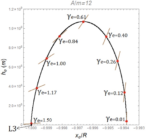
Fig. 4 Black dots represent the solution sets for A/m = 12m2/kg near L3. Red dots are also solutions. The angles γe (in radians) of the normal to the sail relative to the rays of the Sun are shown. Solar rays come from the right side of the figure. The brown straight lines represent the inclination of the planar solar sail (not in scale). The color figure can be viewed online.
Similar patterns can be obtained for other values of the ratio A/m, but other values for the maximum he are reached, as shown in Figure 5. It is interesting to note that different values of the maximum distance from the orbital plane of the Earth are reached in each situation. The equilibrium points take into account the effects of the gravity forces and the solar radiation pressure. Near L3 the gravity forces are weaker, because it is the point located far away from the Earth. Therefore, it is the point where he is larger, compared to the other points, for a given value of the ratio A/m. At points L1 and L2, the gravity forces of the Earth are quite relevant, but the solar radiation pressure effects are weaker at L2. Thus, the point L2 has the smallest values for the maximum he and the middle of the two primaries is the intermediate case for the value he reached. Of course, the values of he increase with A/m for all the points, as expected. These values are quantified in Figure 5. In all the results presented here, the Earth shadow is neglected, because the equilibrium points of interest are not on the orbital plane of the Earth.
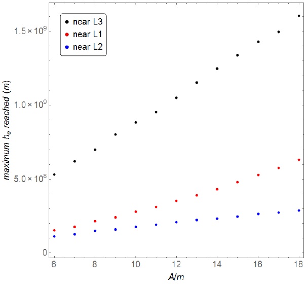
Fig. 5 Color dots represent the solution sets for the maximum value of he reached for different values of the parameter A/m (m2/kg) near L3 (black dots), L1 (red dots) and L2 (blue dots). The color figure can be viewed online.
The next step is to combine those results to obtain geometries that allow the communication between L3 and the Earth. Figure 6 represents the solutions sets for the xe and he coordinates for different values of the ratio A/m. The red line at xe = 0 represents the size of the radius of the Sun. The blue straight line connects the highest point near L3, the point with maximum he, to the highest point reached near the Lagrangian point L1. The green straight line connects the highest point near L3 to the center of the Earth. The values for γe are omitted from this figure for clarity purposes, but each set of solutions contains its respective value for γe.
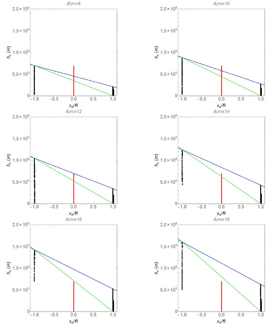
Fig. 6 Black dots represent the solution sets for A/m = 8,10,12,14,16 and 18m2/kg, respectively. The red straight line represents the radius of the Sun. The green straight line connects the maximum value of he reached near L3 to the center of the Earth. The blue straight line connects the maximum value of he reached near L3 to the maximum value of he reached near L1. Note that the solution sets near xe/R ≈−1 form a black column near L3, the solution sets near xe/R ≈ 0.99 form a black column near L1, and the solution sets near xe/R ≈ 1.01 form a black column near L2. These columns are better detailed in Figures 2-4. The color figure can be viewed online.
Figure 5 shows an approximate linear relation between the maximum value for he reached near L1, L2 and L3 as a function of A/m. The results stem from the data obtained by the algorithm used to solve the set of equations that represent the equilibrium conditions. The absolute value of the acceleration of the solar radiation pressure is also proportional to A/m, which means that the maximum he reached is proportional to the absolute value of the force due to the solar radiation pressure. If the reflection of the solar sail is not perfect (a real solar sail), then the resultant force of the solar sail would be smaller for a given ratio A/m, and this linear relation should be considered.
Note that exactly the same results presented in this study could be obtained for z = −he, instead of z = he, due to the symmetry of the problem between “above” and “below” the Ecliptic plane. In fact, there is an infinite number of solutions with the equilibrium point being visible just in the limit of the solar disk, but in any direction (not in the x,z plane). This gives different points of observation for the spacecraft, which can be used to attain different goals of the mission. Besides that, orbits around those artificial equilibrium points are also an option, but these cases are outside the scope of the present paper.
The effects of the interference on the communication signals due to electromagnetic waves as they pass near the Sun are ignored in this work. The calculations are made taking into account that the radius of the Sun is approximately 6.96×10⁸m. Thus, if the value for he near L3 is more than twice this value, the spacecraft can communicate directly with the Earth, and the Sun is no longer an obstacle.
3.1. Communication Solution 1
As mentioned before, three classes of solutions are shown to solve the communication problem. The first of them requires a spacecraft with a ratio areato-mass A/m = 16m2/kg or more, because the spacecraft near L3 placed in the (x,z) plane must have a coordinate in the z axis of at least 1.4×10⁹m to communicate directly with the Earth, as can be seen in Figure 5. Figure 6 (A/m = 16) shows that the green straight line connects the solution point with the highest value for he near L3 to the Earth. This green straight line does not cross the radius of the Sun, thus the spacecraft located in this solution point can communicate freely with the Earth. Figure 7 shows a drawing for this solution.
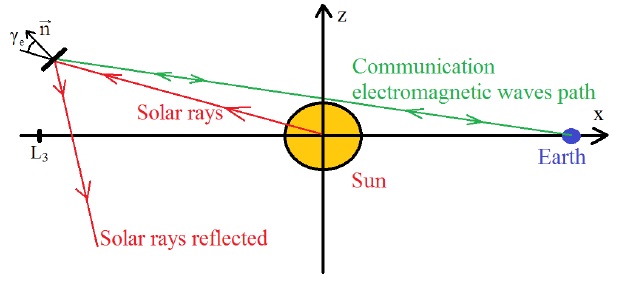
Fig. 7 Geometry of Communication Solution 1. The electromagnetic waves path does not cross the radius of the Sun.
The advantage of this solution is that it is satisfied with just one spacecraft, at the expense of a large area-to-mass vehicle. To have an idea of this ratio, a spacecraft of 100 kg would require an area of 1600m2, which means a square sail with each side measuring 40 meters. The solar sail of the spacecraft for the Ikaros mission had approximately a square 14 × 14m sail (Tsuda et al. 2013).
It is important to mention that a large area for the sail may have some advantages, depending on the goal of the mission. It can be used to obtain solar energy, so reducing or eliminating the need of a power supply. There are also important observations related to the flux of particles in space that require a large collecting surface (Williams 2003). Thus, the effort to build a large solar sail would be used not only to shift the equilibrium point. The values of the parameters and the position of the spacecraft near L3 for this solution are given in Table 2.
3.2. Communication Solution 2
The second alternative to solve the problem uses two spacecraft equipped with solar sails to satisfy the equilibrium condition (equation 7) at very different positions. This kind of solution requires two spacecraft with ratio A/m = 12m2/kg. One of them is positioned at the solution point with maximum he near L3, and the other at the solution point with maximum he near L1. The geometry of this solution is shown in Figure 8.
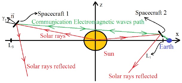
Fig. 8 Drawing of Communication Solution 2. The spacecraft 2 acts as a communication bridge between Earth and spacecraft 1 near L3.
The blue straight line of Figure 6 (A/m = 12) represents the path of the electromagnetic wave used for communication between both spacecraft. This path does not cross the radius of the Sun; both spacecraft can communicate with each other freely. The spacecraft near L1 can communicate with the Earth directly; it works as a communication bridge between the spacecraft located near L3 and the Earth.
This type of solution requires two spacecraft, but each of them with a smaller A/m compared with the first type. Having two spacecraft helps to make observations from two different points in space, which can be interesting for the mission itself, not only to reduce the A/m ratio. On the other hand, it requires two equipments, increasing the costs and the risks of failures. Of course, there is also an infinite number of combinations of solutions of this type, because both spacecraft may not have the same area-to-mass ratio. The best combination depends on other constraints of the mission. This flexibility is interesting for mission designers. The parameters and the position of the spacecraft near L3 and L1 used for this solution are given in Table 3.
3.3. Communication Solution 3
The third kind of solution involves two spacecraft with the same area and mass,
both near L3, positioned as shown in Figure 9. The spacecraft 1 is located above the x axis with the z
coordinate equal to he, and the spacecraft 2 is located symmetrically
opposite below the x axis, with z coordinate equal to −he. The angle
γe of both spacecraft is such that the reflected solar rays go
vertically directly to the other spacecraft, which stays symmetrically opposite
on the z axis, as shown in Figure 9. This
is the reason why the parameter γe is not an independent variable
anymore. In this configuration, both spacecraft can interact through the
reflected solar rays. In this figure, the second spacecraft is subject to part
of the projected area of the first spacecraft over it (and vice versa) and the
total distance of the rays that come from the Sun and are reflected from the
other spacecraft is
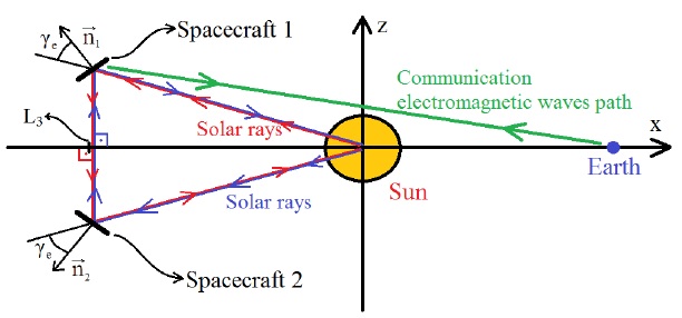
Fig. 9 Drawing of Solution 3. Solar rays that hit each spacecraft are reflected in the direction of the other spacecraft. The resultant force on the spacecraft due to the solar radiation pressure is doubled.
In comparison with the other kind of solutions, Communication Solution 3 demands a considerably smaller ratio A/m, just 9m2/kg, but it also requires an almost perfect planar solar sail in order to achieve a reflection over a distance equal to 2he in the direction of the other spacecraft. In comparison with the first type of solution, for a fixed mass, the area of the solar sail is almost halved. The angle γe must be controlled almost perfectly to ensure that the reflected rays hit the other spacecraft. This kind of solution requires high precision technologies. Table 4 shows the values for the positions and parameters for spacecraft 1 and spacecraft 2, in the configuration of by this third kind of communication solution. The technology for such high accuracy may not be available now, but the idea of the present manuscript is to show this potential possibility for the future, as well as to compare this solution with the two solutions previously shown.
Table 4 Parameters and positions for spacecraft 1 and 2 used in communication solution 3
| Spacecraft 1 (above the x axis): | Spacecraft 2 (below the x axis): | |
| A/m | 9m2/kg | equal to spacecraft 1 |
| xe | −1.49110398621742× 10¹¹ m ≈ −0.997R | equals spacecraft 1 |
| he | 1.45241181117863× 10⁹ m | −1.45241181117863× 10⁹ m |
| γe | 0.780528060797507 | equals spacecraft 1 |
The maximum value of he reached by a spacecraft for a given ratio A/m is significantly increased (almost doubled) for the configuration of Communication Solution 3 in comparison with the previously given solutions, as shown in Figure 10.
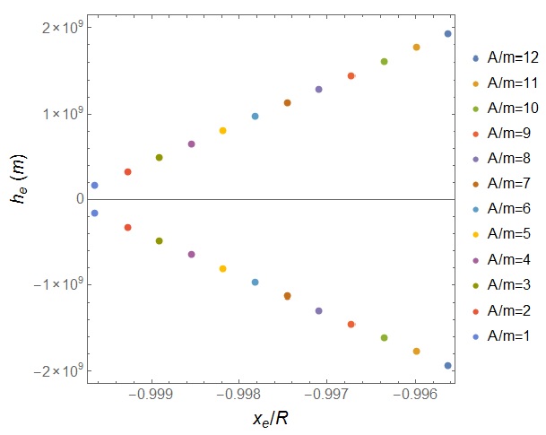
Fig. 10 Color dots are the solution sets in the (x,z) plane represented by the values he and xe/R, for different values of the parameter A/m (m2/kg) near L3 for the Communication Solution 3. The color figure can be viewed online.
This kind of solution uses two spacecraft with the same ratio A/m with symmetry in the z axis with respect to the x axis on the (x,z) plane, enabling both spacecraft to communicate directly with Earth. Solutions in the (x,z) plane with different ratio A/m could also be obtained. For example, the main and heaviest spacecraft (with smallest ratio A/m) could be positioned on an artificial equilibrium point below the x axis, but close to it, and the other spacecraft positioned with a larger value for |he|, such that it could serve as a bridge for communications between the first spacecraft and the Earth. Of course, the exactly positions would depend on all the parameters of each spacecraft, including γe, but this can also allow an interesting flexibility for mission design.
Additionally, this kind of solution is not restricted to spacecraft placed near L3. As an example of an extension of this idea, two spacecraft can be placed around the Earth, one below the Ecliptic plane and the other one symmetrically opposite, above the Ecliptic. The first would have a permanent contact with the region of low latitude, near the south pole, while the other would be in permanent contact with the region of high latitude, near the north pole. The idea of maintaining a spacecraft equipped with a solar sail in permanent contact with high latitude regions of the Earth was first presented and patented by Forward (1991), but the kind of solution presented here takes advantage of two spacecraft with smaller area-to-mass ratio rather than just one, as presented by Forward. The maximum value for he reached is approximately linearly dependent on the ratio A/m, as shown in Figures 5 and 10. The configuration presented in this kind of solution almost doubles the resultant force due to the solar radiation pressure, because equation (14) replaces equation (2) for this configuration. Therefore, the net effect is that the ratio A/m can be almost halved if the objective is to maintain the same value for he, compared to the solutions with a single spacecraft, like that of Forward or Communication Solution 1 presented here. Besides, both spacecraft can be useful, one to interact with regions near the south pole and the other one with regions near the north pole, simultaneously. Figure 11 illustrates the extension of this kind of solution.

4. CONCLUSION
The main purpose of this research is to offer new options of solutions for the communication problem between a spacecraft orbiting the Sun in a point near L3 and the Earth, in the Sun-Earth system. The idea is to take advantage of a large solar sail (which can also be used for other purposes of the mission) to find new artificial equilibrium points, which are not hidden behind the Sun when looking from the Earth. A large number of solutions for each given value of the area-to-mass ratio is found. The results show the exact locations and the attitude of the solar sail for the three collinear equilibrium points.
Three types of solutions are proposed. The first of them uses only one spacecraft, but it requires a large area-to-mass ratio, in the order of 16m2/kg. The second solution uses two spacecraft, each one having a solar sail and located at the artificial equilibrium points near L3 and L1. For this type of solution a ratio A/m = 12m2/kg is enough to obtain communication. The third kind of solution requires a considerably smaller area-to-mass ratio (A/m = 9m2/kg). This solution presents high precision technological challenges, but this manuscript aims to show its potential for the future, not considering the details of implementations.
In this way, three options for solutions are shown. Overcoming the negative aspect of the communication problem, the point L3 can be considered for practical applications, while the other two unstable collinear points (L1 and L2) could be considered in the future.
Of course, this is a preliminary study, and more sophisticated models for the solar sail should also be used to improve the results obtained here. Specific models, including other perturbations, should also be used to calculate new sets of solutions for the three types of communication solutions presented in this research.

