


 nueva página del texto (beta)
 Inglés (pdf)
 Artículo en XML
 Referencias del artículo
 Enviar artículo por email
 Citado por SciELO
  Similares en
SciELO
Similares en
SciELO 
 Permalink
1. INTRODUCTION
In recent decades, thousands of satellites were launched for climate monitoring, telecommunications, remote sensing, global positioning systems, scientific research and many other applications. In 2016, over 17,000 objects in orbit were present, most of them being space debris. According to the re port of the Inter-Agency Space Debris Coordination Committee (IADC), (IADC 2002), space debris are all non-functional artificial objects, including frag ments orbiting the Earth or re-entering the atmo sphere. Due to the increase of the space debris, and the problems related to this process, the space agen cies ESA (Europe), NASA (USA), JAXA (Japan), CNES (France) and the IADC have issued documen tation to regularize practices that limit the growth of space debris in some regions of interest, such as the regions of Low Earth Orbit (LEO), Geosynchronous Orbit (GSO) and the orbit of the Global Navigation Satellite System (GNSS) (Hull 2011). Thus, IADC (2002) and the U.S. Government (1997) defined 25 years as the time limit after which a satellite in the LEO region has to be removed. NASA (1995) determined that satellites at their end-of-life phase and the upper stages of launchers for the GPS constellation should be moved to an orbit 500 km above or below their nominal orbits. However, this disposal strategy is not entirely satisfactory, because these orbits are potentially unstable due to the presence of the 2:1 resonance between the argument of the perigee and the longitude of the ascending node of the satellite orbit, whose main effect is an increase in the satellite eccentricity. This resonance acts whenever the satellite inclination is near 56 degrees, regardless of the semi-major axis (Gick 2001; Chao & Gick 2004; Sanchez et al. 2009). This poten tial increase of the eccentricity may cause the dis carded satellite to cross the orbit of other satellites, thus increasing the risk of collisions with operational satellites.
In the present work, we propose the use of controlled solar radiation pressure, (where the area-to-mass ratio and/or the reflectivity coefficient varies between maximum and minimum values) to change the orbital energy of the discarded satellite, to cause its de-orbiting. More specifically, when the satellite is moving in the direction of the Sun, the proposed control will cause the perturbation due to the solar radiation pressure to have the maximum value and, when the satellite is moving in the opposite direction, the pertubation due to the solar radiation pressure will have its minimum value. To use this technique it is necessary to have a device that can modify the area-to-mass ratio and/or the reflectivity coefficient of the satellite. Small values for the area-to-mass ratio and/or the reflectivity coefficient are considered. In some cases it may not be necessary to modify the area of the satellite to achieve the de-orbit. Satellites in near circular MEO with arbitrary inclination are considered, so the idea of sending the satellite to de-orbit is replaced by the concept of sending it to a graveyard orbit. The reason for this the long time required to reach the atmosphere of the Earth from a MEO using this technique.
The evolution of the orbit strongly depends on the initial values of the argument of periapsis and on the longitude of the ascending node, due to the 2:1 perigee longitude of the ascending node resonance (2w + Ω), as mentioned before. Then, it is important to find initial conditions of w and Ω that lead to trajectories with minimum eccentricities. The natural precession of the orbits changes the values of those two elements. Therefore, after finding the values for those two orbital elements that reduce the maximum eccentricity, it is possible to wait for an ideal moment to start the control, such that the maximum eccentricity is minimized.
In this work we also develop an analytical model to find the maximum eccentricity reached for differ ent initial conditions for the argument of perigee and for the longitude of the ascending node. After finding the best initial conditions, the orbits are propagated using a numerical model, with the inclusion of other forces. The advantage of this analytical model is that we can save computational time when finding initial conditions for w and Ω, since the analytical model is considerably faster than the numerical model.
2. REVIEW OF THE LITERATURE
Looking back in time, Jenkin & Gick (2001, 2002, 2005, 2006), showed that a satellite with inclination near 56 degrees in the GNSS region could be potentialy unstable, due to the 2w + Ω resonance. This resonance can cause a growth of the eccentricity, making a discarded satellite cross the orbit of active satellites of this constellation. The authors also analyzed the risk of collisions between operational and discarded satellites. These studies showed that there is a low probability of collisions. However, the collision probability increases with the eccentricity, especially considering that, in the long term, the region will receive many other satellites and upper stages of launchers. Therefore, the collision probability can increase considerably (Pardini & Anselmo 2012). Furthermore, even small probabilities need to be taken into account, because of the catastrophic effects caused on a mission by a collision.
Therefore, disposal techniques that remove the satellite to orbits closer to the nominal ones are not a final solution for this problem. Another option is the so called "de-orbit". According to IADC (2002), de-orbit is an intentional change in the orbit of a satellite (or other space objects, such as launch vehicles) to place it in an orbit that forces it to reenter the atmosphere of the Earth, thus eliminatating the risks of collisions with other satellites. This pro cess is usually done through the use of propulsion systems, which spend fuel. Lucking et al. (2011) presented a strategy to de-orbit a satellite using so lar radiation pressure to increase the eccentricity of the orbit, in order to place the perigee inside the atmosphere of the Earth. To perform this task, the use of an inflatable balloon-type device was consid ered. The advantage of this device is that it does not need attitude correction maneuvers during de orbiting, because it has a spherical shape when inflated. Lücking et al. (2012a) considered in their study the solar radiation pressure and the J 2 coefficient of the geopotential. Note that, for orbits between 20,000 and 35,000 kilometers of altitude and low inclinations, the whole process takes at least 5 years, using an area-to-mass ratio of 50 m2/kg. For Molniya type orbits, the required area-to-mass ratio would be 1 m2/kg. Lücking et al. (2012b) focused on the use of area augmentation devices for heliosyn-chronous orbits with high altitudes.
Guerman & Smirnov (2012), studied single im pulsive maneuvers and considered satellites with attitude control by spin stabilization and passive stabilization using the magnetic field of the Earth. They analyzed de-orbiting with the use of propellant thrusters and area augmentation devices. Using the same type of attitude control, Trofimov & Ovchin-nikov (2013) studied de-orbiting with low thrusters.
Romagnoli & Theil (2012) studied the use of a solar sail to de-orbit a satellite from the LEO region. The study also considered the attitude of the solar sail. The authors simulated the de-orbit for a he-liosynchronous satellite with 140 kg using a 25 m2 solar sail. For an initial altitude of 450 km, the de-orbiting lasted less than 20 days and, with an initial altitude between 600 and 650 km, the de-orbiting lasted between 350 and 400 days.
Alessi et al. (2014) made a survey of satellites, both in operation and deactivated, for the GNSS constellations in the year of 2013. They presented the current methods of disposal of these satellites, which mostly consist in sending the satellite or the launching upper stage to be removed to orbits 500 km above or below their nominal orbits (NASA 1995). The study considered a complete de-orbit when the perigee altitude was below 200 km. The first method uses low thrusters that, depending on the fuel consumption, accomplish the de-orbit to in between 2.5 and 25 years. The second method pre sented in their study is based on using the solar ra diation pressure and an area augmentation device. For the de-orbit to occur in 5 years, depending on the altitude and inclination within the MEO region, a maximum area-to-mass ratio between 11.4 and 12.1 m2 /kg is needed. The combined use of an increasing area device and low thrust propulsion decreases the fuel consumption by 40-50%.
Sanchez et al. (2015) considered the disposal of satellites in the resonance 2ꞷ+Ω by choosing the initial conditions of the disposal orbit. As already mentioned, this resonance influences the eccentricity of the orbit and defines regions of maximum and minimum growth of the eccentricity, depending on the initial eccentricity and on the initial values of ꞷ and Ω. This study defines two strategies: find regions of minimal growth of eccentricity, or initial conditions where the growth of the eccentricity, due to the resonance 2ꞷ+Ω, will lead to a perigee height below 200 km, thus causing the de-orbit. The au thors also use maneuvers to increase the apogee, in order to increase the eccentricity so that the reso nance 2ꞷ+Ω will occur in less time, compared to the nominal apogee.
Forward et al. (2000) studied de-orbit in the LEO region using an electrodynamic space tether. This type of tether uses the interaction of an electrical current passing through a cable (which connects two bodies that are in different orbits) with the magnetosphere. This interaction generates a force oppo site to the motion of the satellite, called electrodynamic drag, which causes the decay of the orbit of the satellite. The device considered in this study has a mass smaller than 3% of the mass of the satellite. The study found that the region between 700 km and 2, 000 km of height is ideal for the use of this equip ment. Yamagiwa et al. (2001) studied de-orbit for elliptical orbits, also with the use of an electrodynamic tether. Its use reduces the de-orbiting time, in some cases from 10 years to only a few months. Ahedo & Sanmart-egrave (2002) analyzed the relationship between the length of the cable used and the time required for de-orbit. They noted that an increase of the cable increases the electrodynamic drag and, consequently, the time to de-orbit the satellite will be smaller. According to Pardini et al. (2009), the advantage of using electrodynamic tethers is that it saves the use of propellant thrusters. A discard via propellant requires 10% to 20% of the total weight at launch, whereas the tether electrodynamic devices weights are between 30 and 50 kilograms, so they can achieve de-orbit using only 1% to 5% of the launch mass.
Janhunen (2010) proposed another method of de-orbit similar to the electrodynamic tethers, but with a different physical principle. This study considered a device which uses the electrodynamic drag generated by the interaction of the ionospheric plasma with a negatively charged cable. There are other types of devices that can be used to de-orbit a satellite. Viquerat et al. (2014) showed a simi lar device with an inflatable sail that, when inflated, becomes rigid. Then, the de-orbit occurs due to the atmospheric drag. These aspects limit its use to low orbits. Its ideal use would be to de-orbit CubeSats. Furumo (2013) discloses an alternative form of de-orbit, using cold gas thrusters, which have optimal use in the de-orbit of CubeSats.
Although there are many types of devices that can be used for the de-orbit, this study focuses on devices that use controlled solar radiation pressure. The effect of the solar radiation pressure on the motion of artificial satellites has been studied for a long time. Parkinson et al. (1960) noted that the satellite type ECHO-1 balloon, at an altitude of 1,600 kilome ters, was shifting about 6 km per day, and the satel lite Beacon was moving only about 1 km per day. In resonant conditions, the effect accumulates and the satellite can have its lifetime reduced. The discrepancy between observation data and the perigee calculated for the satellite Vanguard I led Musen et al. (1960) to study the effects of solar radiation pres sure on this satellite. The inclusion of solar radiation pressure in the model gave results much closer to the observed ones, except for short-term effects. Musen (1960) made a more detailed analytical study on the effects of solar radiation pressure on the satel lite Vanguard I. Wyatt (1961) studied the effects of solar radiation pressure on the secular accelerations of the satellite and compared solar radiation pressure with atmospheric drag. At high altitudes, with low atmosphere density, the solar radiation pressure became very important. Bryant (1961) developed an analytical model for calculating the osculating el ements, but his model neglected the effects of the shadow of the Earth in the motion of the satellite. After that, Kozai (1963) developed an analytical model which considered the effects of the shadow of the Earth. Later, Adams & Hodge (1965), in their study about the effects of solar radiation pressure on the satellite, explained the physical mechanism of the increase of the eccentricity and gave special attention to the resonances related to it. Lala & Sehnal (1969), and later Ferraz-Mello (1972), made more detailed studies on the effect of the shadow of the Earth on the perturbation caused by the solar radia tion pressure. Krivov & Getino (1997) analyzed the impact of solar radiation pressure on the eccentricity of the orbit of a satellite with large area-to-mass ratio and high altitudes. Moraes (1981) developed a semi-analytical model combining the effects of solar radiation pressure and atmospheric drag on an artificial satellite. Valk & Lemaître (2008) and Hubaux & Lemaître (2013) and Hubaux et al. (2013) studied the effects of solar radiation pressure on the orbital stability of space debris. Recently, Deienno et al. (2016) studied the use of controlled solar radiation pressure to the de-orbit a satellite.
3. ANALYTICAL STUDY
For simplicity, the analytical model considers the solar radiation pressure and the oblateness of the Earth, so that lunar and solar perturbations are not taken into account. For simplicity, the shadowing effect is neglected, since we are working with high orbits. Another simplification is to ignore the obliquity of the Earth ε = 23.45 degrees. Those simplifications may look to strong at first, but the numerical results will show that the analytical model developed here is appropriate to predict the eccentricity behavior.
To describe the evolution of the orbit we use the set of slowly changing modified equinoctial elements (p, f, 9, h, k, L), where p = α(1 - e2) is the semilatus rectum of the elliptical orbit. These elements are:
where θ = u -ꞷ is the true anomaly (see Walker, 1985). The variational equations for these elements have the form:
where µ is the geocentric gravitational constant, s2 = 1+h2+k2, and w = p/r = 1+f cosL+g sinL. The vector ∆ = (∆t,∆r,∆n) is the acceleration caused by the solar radiation pressure and the J2 effect. Its tangential, radial, and normal components are given by:
where
and
The control device increases the area/mass ratio of the satellite (parameter P) whenever the angle between the position vector of the Sun r ⊙ and the position vector of the satellite r, both centered on Earth, is less than 180o and the satellite moves towards the Sun. This leads to the following form for the acceleration caused by the solar radiation pressure:
where P1 > P0.
In the frame of the problem of satellite disposal, it is necessary to choose a control law that reduces the semi-major axis a of the orbit of the satellite. To start the analytical development of the problem, a near circular MEO (α ≈ 25,000 − 30,000 km) is considered. We shall study the phase of disposal assuming that e ≪ 1 and p ≈ r ≈ a. Since ∥∆∥ is rather small, we have:
Under these hypotheses, retaining only the main terms from equations (1) - (3) we get:
Integrating equations (9)-(11), the change of the elements p, f, and g over the entire orbit is given by:
Observe that
and
Therefore the average rates of change of the orbital elements are given by the following equations:
From equation (12) it follows that p always decreases. After some simple calculations, from equations (13) and (14), we obtain:
From this we have:
In MEO, the elements p, Ω, and ω vary slowly in comparison with λ⊙. For example, during the period of one year, we can approximately consider these elements as constants. Therefore we get
where Λ⊙ = dλ⊙/du and u ∈ [0,2π]. This equation can be used to analytically evaluate the evolution of the eccentricity during one year.
It is necessary to validate the analytical model, and a numerical model is used. The equations of motion of the satellites in this model are given by:
where r is the position vector of the satellite and µ is the gravitational parameter of the Earth. P G is the perturbation due to the geopotential up to degree and order 8, as in previous studies in the region of the GNSS (Hugentobler 1998; Ineichen et al. 2003; Chao & Gick 2004; Beutler 2005). P S and P L are the perturbations from the Sun and the Moon, respectively. P SRP is the perturbation due to the solar radiation pressure and it is given by:
where P⊙ is the solar radiation pressure, determined by the solar flux at 1 AU. P⊙ is considered constant in the neighborhood of the Earth, so P⊙ = 4.56 × 10⁻⁶Nm−2. ν is the shadow function (Montenbruck & Gill 2000), where ν = 1 when the satellite is completely exposed to the sunlight, ν = 0 when the satellite is completely covered by the shadow of the Earth (umbra), and 0 < ν < 1 when the satellite is in the penumbra. AU is the average distance Earth-Sun and r⊙ is the distance Sun-satellite. For this study, the main terms of the equation for the radiation pressure are the coefficients of reflectivity (Cr) and the area-to-mass ratio (A/m). With these assumptions, the latter two terms appear as a product; then the variable used is α = Cr A/m, thus one can use different reflectivity coefficients combined with several values of the area-to-mass ratio in the following simulations.
4. RESULTS
Initially, using the most complete numerical model, it is necessary to show the importance of the use of the control given by Equation 7 to generate the orbital decay. Figures 1 and 2 are obtained using a semi-major axis equal to 26,000 km, 0.02 for the eccentricity and an inclination of 10 degrees. The argument of perigee, longitude of ascending node and mean anomaly are all equal to 0 degrees. In both figures, the minimal value of α used is equal to 0.03 m2/kg. For all simulations in this paper, α0 = 0.03 m2/kg, which is a typical value for GNSS satellites. Figure 1 shows the case without control. Figure 2 represents the evolution of the orbit of the satellite in a situation where control is not used, but α is fixed at 1.5 m2/kg. In this situation, the device changes α from 0.03m2/kg to 1.5 m2/kg and this value was kept fixed. We can see in these figures that, without the use of a control, there is no decay of the satellite within the simulated period.
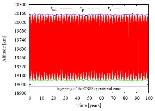
Fig. 1 Evolution of the satellite position (r), perigee (rp) and apogee radius (ra) over 100 years, without control and with α fixed at 0.03 m2/kg. Initial conditions are: semi-major axis 26,000 km, (which means an altitude of 19,101.8634 km), eccentricity 0.02, inclination 10 degrees. Perigee argument, longitude of the ascending node and mean anomaly are all equal to 0 degrees.
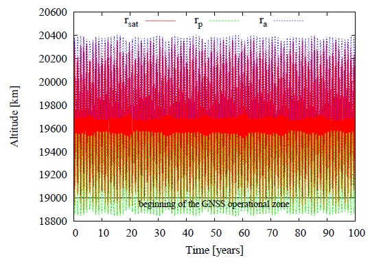
Fig. 2 Evolution of the satellite position (r), perigee (rp) and apogee radius (ra) over 1 year, without control and with α fixed at 1.5 m2/kg. Initial conditions are: semi-major axis 26,000 km, (which means an altitude of 19,101.8634 km), eccentricity 0.02, inclination 10 degrees. Perigee argument, longitude of the ascending node and mean anomaly are all equal to 0 degrees.
Using equation 17, we can analytically evaluate the evolution of the eccentricity of the satellite over one year. Then, it is possible to find regions where the eccentricity reached large amplitudes in its variation, during one year, and the opposite situation, where the eccentricity reached small amplitudes. Since to minimize the risk of collision during the decay it is desirable for the satellite to have a low variation in its eccentricity, equation 17 is used to find the initial conditions for ω and Ω to start the de-orbiting. Then, the evolution of the eccentricity is mapped, and the maximum values for different initial conditions of the argument of perigee (ω) and longitude of the ascending node (Ω) are found. Figures 3a and 3b show the differences between the results for the analytical model (Figure 3a) and the numerical model (Figure 3b). The initial conditions of Figures 3a and 3b refer only to the semi-major axis, eccentricity and inclination of the orbital plane, as defined in the captions of Figures 1 and 2. However, in this case, a control device is used, increasing and decreasing the area and/or the reflectivity coefficient, up to the maximum value of α, which is equal to 1.5 m2/kg. The results of Figures 3a and 3b show that there is a good compatibility between the analytical and numerical results, which validates the assumptions made to derive the analytical equations.
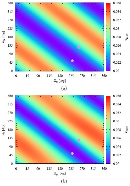
Fig. 3 Maximum eccentricity reached in one year using a control device. The initial conditions for semi-major axis, eccentricity and inclination are the same ones used in Figures 1 and 2. (a) Results obtained from the analytical model (equation 17). (b) Results obtained using the numerical model. The color figure can be viewed online.
From Figures 3a and 3b, two different points are chosen to show the evolution of the eccentricity over on year for the analytical and numerical models. These points are chosen because they represent the best and the worst cases of the comparison of analytical and numerical results. They were found by taking the difference between the maximum eccentricities reached using the analytical and the numerical models (Figures 3a and 3b). These cases are shown in Figures 4a and 4b. The initial conditions of Figures 4a and 4b refer only to semi-major axis, eccentricity and inclination of the orbital plane, as defined in the captions of Figures 1 and 2. Figure 4a was made for the best match between the analytical and numerical models (gray circle shown in Figures 3a and 3b. The argument of perigee is equal to 54 degrees and the longitude of the ascending node is equal to 232 degrees. One can note that there is a good agreement between analytical and numerical models. Figure 4b, which is made for the worst agreement, shows that there is a shift between the curves (purple circle marked in Figures 3a and 3b, where the argument of perigee is equal to 124 degrees and the longitude of the ascending node is equal to 258 degrees. Analyzing the results, this gap in the curves is evident. Since equation 17 of the analytical model was developed considering semi-major axis, argument of perigee, longitude of the ascending node and inclination of the satellite orbit as constants, it is expected that, in some cases, the gap would occur. However, although there is a difference in the prediction of the evolution of the eccentricity, there is a very good agreement in terms of finding the maximum values, which is the goal of the present research. The results presented here also allow to find the initial conditions, in terms of the argument of perigee and the longitude of the ascending node, to start the decay, taking into account the maximum eccentricity reached by the orbit of the satellite within one year. They can be obtained from grids made using the analytical model of evolution of the eccentricity, as shown in Figures 3a and 3b. Thus, to validate the analytical model, one more grid was made, similar to the ones made in Figures 3a and 3b.
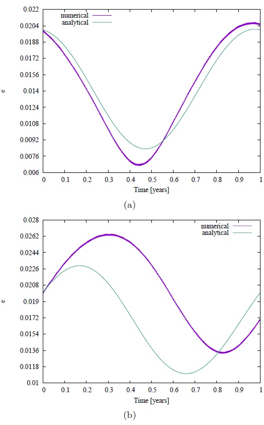
Fig. 4 Evolution of the eccentricity in one year, for the same initial conditions of Figure 3a. (a) For the gray circle marked in Figures 3a and 3b, where the argument of the perigee is equal to 54 degrees and the longitude of the ascending node is equal to 232 degrees. (b) For the purple circle marked in Figures 3a and 3b, where the argument of perigee is equal to 124 degrees and the longitude of the ascending node is equal to 258 degrees.
Figures 5a and 5b are obtained for the same initial conditions used in Figures 3a and 3b, except for the inclination, which in this case is considered to be 56.06 degrees. This value is already close to the actual values of the satellites of the GNSS, located in MEO region. Although the analysis of resonances is not within the scope of this study, the chosen value is the critical inclination for the resonance 2ω+Ω (Sanchez et al. 2009). Figures 5a and 5b are obtained using the analytical (equation 17) and the numerical model, respectively. Again, there is a good agreement between the two models. The regions of maximum and minimum eccentricity are the same in both models, and the maximum and minimum values of the eccentricity are also the same. The value 0.034 is the maximum value for the eccentricity and 0.02 is the minimum, during one year. Except for minor differences, the maximum and minimum regions are located on the same diagonal. It is important to remember that these differences are expected, due to the simplification of the analytical model, which considers as constants over one year all the orbital elements, except the eccentricity.
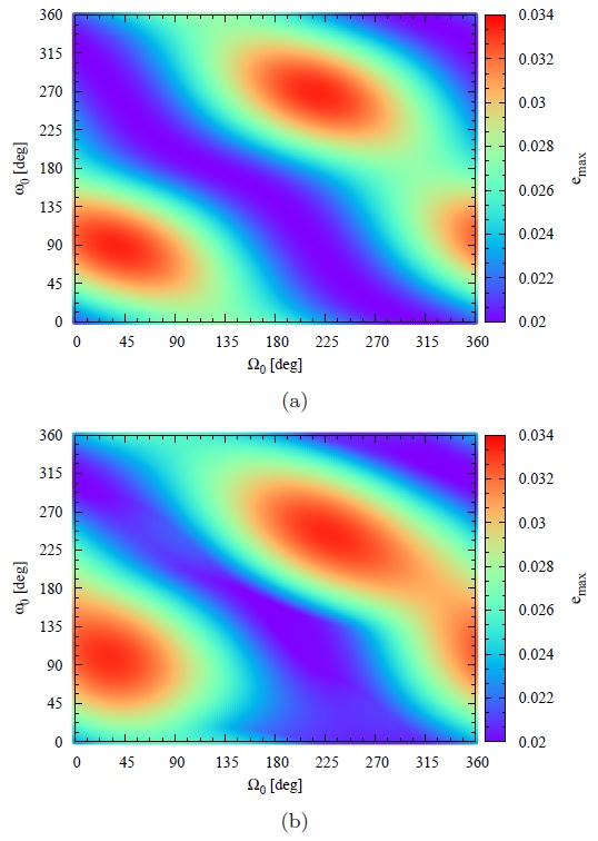
Fig. 5 Maximum eccentricity reached over one year using a control device, for the same initial conditions used in Figures 3, but with an inclination equal to 56.06 degrees. (a) Results obtained from the analytical model (equation 17). (b) Results obtained using the numerical model.
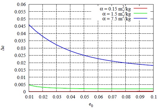
Now, a final test is made to show the validity of the analytical model for different initial values of the eccentricity (e0) and α. For a better comparison of the results shown in Figures 4a and 4b, the average over one year of the magnitude of the differences of all trajectories (which are single points in these figures) is obtained for each initial value of the longitude of the ascending node and argument of perigee. Equation 18 better shows this definition:
where n is the total number of points of the trajectory in one year, ea and en are the eccentricities obtained by the analytical and numerical models, respectively, for the same point of the trajectory (or time instant).
Figure 6 is obtained using equation 18, with the same initial conditions used in Figure 4b, but for different initial values of the eccentricity. The curves are drawn for values of α equal to 0.15 m2/kg, 1.5 m2/kg and 7.5 m2/kg, respectively. In this analysis it is possible to notice that, when the initial eccentricity is increased, the analytical model gives better results for larger values of α. It is also possible to see that, for values of α up to 1.5 m2/kg, the error is small for initial eccentricities above 0.02. This is important, because the satellites in the GPS region have eccentricities equal to or above this value, due to the orbital resonances in the region. It is expected that the satellites currently being launched will also reach these values (Gick 2001; Sanchez et al. 2015). α equal to 7.5 m2/kg is a very high value, used to see the effects of this parameter, but it is not expected that devices of this size will be implemented in real missions.
After validating the analytical model, we can use it to generate grids of maximum eccentricity reached during one year of evolution. Thus, using the analytical model instead of the numerical model, one can save a huge computational effort to generate grids. While a grid made using the numerical model takes a few days to be completed, the one made from equation 17 of the analytical model is finished in a few seconds, given the same computational conditions in terms of hardware and software.
Figure 7 shows the maximum eccentricity reached by the orbit of the satellite during the decay over one year. This case has been computed using the initial conditions of an actual GNSS satellite at the epoch August 01, 2016. The satellite considered, which belongs to the GPS constellation, is the BIIR-5. The initial conditions are: semi-major axis equal to 26,559.8671875 km, eccentricity equal to 0.0199945, inclination equal to 56.6962 degrees and mean anomaly equal to 51.704 degrees. Note that the minimum value for α is 0.03 m2/kg and the maximum value is 1.5 m2/kg. Figure 7 shows that the maximum value reached by the eccentricity is 0.034. As in previous cases (Figures 3a, 3b, 5a and 5b), the eccentricity did not exceed its initial value in the regions of its minimum growth (blue region of Figure 7).
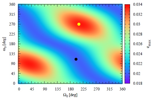
Fig. 7 Maximum eccentricity reached over one year based on equation 17. Initial conditions are: semi-major axis equal to 26,559.8671875 km (which means an altitude of 19,859.28784969188 km), eccentricity equal to 0.0199945, inclination equal to 56.6962 degrees and mean anomaly equal to 51,704 degrees, α minimum of 0.03 m2/kg and α maximum of 1.5 m2/kg. The color figure can be viewed online.
Figures 8a and 8b consider the black circle marked in the region of minimum eccentricity in Figure 7, where the argument of perigee is equal to 110 degrees and the longitude of the ascending node is equal to 200 degrees. Figure 8a shows the variations in the satellite position (r), the perigee radius (rp) and the apogee radius (ra) for a satellite leaving the operating zone of the GNSS between an altitude of 19,000 and 24,000 km, with approximately 2.5 years of simulation. Figure 8b shows the variation of the eccentricity, explaining what was shown in the grids. The values of the eccentricity do not exceed the initial value during the simulation time considered. One can note that, in the first 5 years of simulation, there is a tendency for the circularization of the orbit. However, in longer simulations, this bias may not exist.
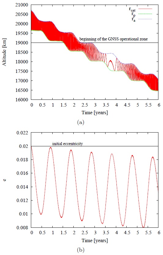
Fig. 8 Simulation for the black circle marked in the region of minimum eccentricity shown in Figure 7, where the argument of perigee is equal to 110 degrees and the longitude of the ascending node is equal to 200 degrees. (a) Satellite position evolution (r), perigee radius evolution (rp) and apogee radius evolution (ra). (b) Eccentricity evolution.
Figures 9a and 9b represent the yellow circle marked on the region of maximum growth of the eccentricity shown in Figure 7. The argument of perigee is equal to 270 degrees and the longitude of the ascending node is equal to 210 degrees. Figure 9a shows the evolution of the satellite position (r), perigee radius (rp) and apogee radius (ra). It shows that the satellite takes about 3.5 years to leave the GNSS operational zone, a year longer compared to the situation of minimum eccentricity (Figure 8a). Figure 9b shows the variation of the eccentricity from the very beginning of the simulation, which explains the longer time the satellite needs to leave the operational zone (Figure 9a).
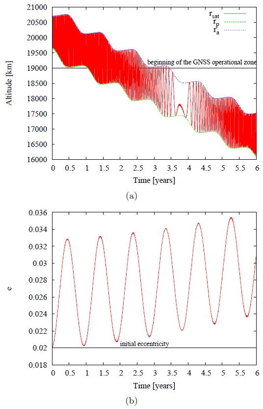
Fig. 9 Simulation for the yellow circle marked on the region of maximum growth of eccentricity of Figure 7, where the argument of perigee is equal to 270 degrees and the longitude of the ascending node is equal to 210 de grees. (a) Satellite position evolution (r), perigee radius (rp) and apogee radius (ra). (b) Eccentricity evolution. The color figure can be viewed online.
From the results presented here, we can conclude that the regions of minimum peaks of the eccentricity are ideal for the orbit decay of a satellite based on the increase of the area and/or the variation of the reflectivity coefficient. It is known that precession of the argument of perigee and longitude of the ascending node in the orbits of the GNSS satellites are present, so it would be possible to achieve the required initial conditions without the use of extra maneuvers. It is only required to wait for the correct time to start the process, and it is possible to avoid repositioning maneuvers.
5. CONCLUSION
The goal of the present paper is to search for trajectories with minimum eccentricity to send a satellite to a graveyard orbit with the help of solar radiation pressure. The idea is to cause a controlled decay of the satellite by making a variation of the area-to-mass ratio and/or the reflectivity coefficient of the satellite. This control can remove energy from the satellite, forcing a decay to a graveyard orbit, which is an orbital region different from the operational zone.
An analytical model was derived to find the maximum eccentricity reached during the removal tra jectory for different values of the initial conditions, which are the argument of perigee and longitude of the ascending node. Essentially, with the best values for those two orbital elements, it is possible to wait for the best moment to start the control, such that the maximum eccentricity is minimized. It is important to find trajectories with minimum eccentricities because, in this case, the satellite travels in narrow orbital regions, and the risk of collisions with other satellites is reduced.
The analytical model was validated using the numerical model, which includes more perturbing forces. The results show that the analytical expres sions can make a very good estimation of the max imum eccentricity achieved by the satellite. Thus, this analytical model is useful in the design of dis posal orbits for satellites.

