


 nova página do texto(beta)
 Inglês (pdf)
 Artigo em XML
 Referências do artigo
 Enviar este artigo por email
 Citado por SciELO
  Similares em
SciELO
Similares em
SciELO 
 Permalink
1. INTRODUCTION
Recently a new type of protoplanetary disks has been classified as pre-transitional disks; they show emission of optically thick hot dust near the star and a gap (Espaillat et al. 2007, 2010; Kim et al. 2013). These disks are complementary to the wellknown transitional disks, which have holes in their inner parts with optically thin emission from hot dust (Calvet et al. 2005). Both disk types show a mass accretion rate onto the star of about ≈ 10−10 to 10−8 M⊙/yr (Calvet et al. 2002, 2005; Close et al. 2014; Espaillat et al. 2007, 2008; Najita et al. 2007), and regions with holes or gaps with sizes around tens of AU (Andrews et al. 2011; Brown et al. 2009; Espaillat et al. 2010; Quanz et al. 2013).
An indirect way to infer the presence of planets or their possible mechanisms of formation is through observations of the dust and gas in disks (Chauvin et al. 2005; Lagrange et al. 2010). Photometric observations with Gemini by Boccaletti et al. (2013)) show multiple spiral patterns of the transitional disk HD 100546. Their observations suggest that these patterns are produced by gravitational perturbations due to the presence of planets in the inner regions of the disk. Using the Very Large Telescope Interferometer, the Keck Interferometer, Keck-II, Gemini South, and IRTF, Kraus et al. (2013) spatially resolved asymmetries in the gap region of V1247 Ori, which suggest the gas is perturbed by hypothetical planets in the gap. A feasible way to explain the cavity region in transitional and pre-transitional disks is through planetary accretion. This problem was previously addressed by Zhu et al. (2011), who concluded that the dust-to-gas ratio must be 3 orders of magnitude smaller than the standard value, 1:100, in order to explain the existence of the cavity.
More recently, Bruderer et al. (2014) resolved observationally the cavity of Ophiuchus IRS 48 with ALMA. They found gas structures inside the 20 AU dust cavities, suggesting that this behaviour cannot be explained by gas photoevaporation, and pointing to a cavity cleared by planets. Perez et al. (2014) found asymmetries in ALMA observations of the transitional disks SAO 206462 and SR 21. They modelled the cavity including a variable mass surface density, with a steady-state vortex described as a Gaussian in the radial and azimuthal directions. They found that the asymmetrical component of the emission (20%), can be explained by material inside the asymmetry with a mass of the order of 2 Jupiter masses. Dodson-Robinson & Salyk (2011) studied the formation of structures inside the hole; they concluded that the planetary system induces the formation of structures in the gap. These structures consist of currents (like filaments) and an optically thick residual inner disk. Dodson-Robinson & Salyk showed that the currents can be optically thin or thick. Particularly, the optically thick gap structures can live in an optically thin environment, suggesting that the optically thick regions can hide disk material.
In order to address the problem of hidden material in optically thick regions of the disk and, in general, to describe the configuration of material inside the disk due to immersed planets, we run a set of models to detect structures in the protoplanetary disks for several optical depths ranges in hydrodynamical simulations. From the simulations, we extract the contribution of mass, density and area for each structure. Our algorithm is able to calculate the spectral energy distribution (SED) for each structure in the cavity. To test our algorithm, we use the same initial conditions as Zhu et al. (2011), which restrict us to consider well-coupled dust and gas.
Summarizing, in this work we address the problem of hidden material in the cavities and propose the interaction of the planets in the disk as the responsible mechanism for opening gaps and creating structures inside. This paper is organized as follows: In § 1 we introduce the protoplanetary disks with gaps and structures. In § 2 we present a set of hydrodynamical simulations of a protoplanetary disk with an embedded planetary system. For each simulation we characterize the structures inside the formed gap, such as the number of structures, their masses and sizes, and the filling factor. Also, we describe a method to extract a spectrum associated to these structures. Finally, we propose a disk model and a planetary configuration to explain the SED of the stellar system V1247 Ori (Kraus et al. 2013). In § 3 we show the results. In § 4 we present the discussion. In § 5 we point out the conclusions.
2. METHODOLOGY
The presence of a planetary system embedded in a protoplanetary disk creates a gap around each planetary orbit (Lin & Papaloizou 1986; Crida et al. 2006). We hypothesize that when there are overlapping gaps because of the proximity of the planets, a larger gap is produced with a lot of structure. A structure is defined as a region with a clearly lower or larger density with respect to its surroundings. Each structure is characterized by its optical thickness; in particular an optically thick structure is able to hide gas and dust, in the sense that this material does not have a contribution to the spectrum. From a hydrodynamical simulation one is able to extract the amount of material that is hidden inside this kind of structures, even when they do not have a counterpart in the SED. In this section, we present the initial conditions for a set of hydrodynamical simulations of a protoplanetary disk with an embedded planetary system, aiming to obtain the information that characterizes the system: their size, mass and spectrum. We realize that this set is just a small sample of all the possible configurations for the system. However, this is a preliminary study that clearly shows the richness of the structures immersed in the gap, and it will become very handy in a detailed analysis of the disk structure of observed systems as a first step to face their modelling.
Our simulations are developed by the hydrodynamical code for planetary migration FARGO1(Masset 2000). This code uses a van Leer upwind algorithm on a 2D staggered mesh with centre in a fixed primary. In order to increase the time-step at each radius, the Courant-Friedrichs-Lewy (CFL) condition is always satisfied. An orbital advection scheme on the average azimuthal velocity at each radius has been implemented to reduce the numerical diffusivity. The procedure follows FARGO ‘Fast Advection in Rotating Gaseous Objects’ manual. This implementation decreases the required time by one order of magnitude. The code solves the NavierStokes and continuity equations for a Keplerian disk with embedded protoplanets. Disk and planets are influenced by the gravitational potential of a central star. The gas is not subject to auto-gravity. The Courant number is fixed at 0.5. The code contains the viscous stress tensor which is implemented in the Navier-Stokes equations and uses an artificial viscosity of second order (see the (33) and (34) equations of Stone & Norman 1992). We note that among the grid based and SPH codes, FARGO is the fastest (see de Val-Borro et al. (2005)).
2.1.1. Hydrodynamical Simulations
In order to define a set of cases in which an analysis of the formation of structures inside a gap carved by a planetary system can be done, we choose the cases analysed in Zhu et al. (2011). According to Crida et al. (2006), the main parameters that affect the gap shapes are the disk thickness, the planetary mass and the disk viscosity. These parameters are included in the following general criteria:
for the gap formation, where the first left term is a thermal-gravitational criteria (Ward et al. 1997), the second left term is a viscous-gravitational criteria (Artymowicz et al. 1994). In the first term, H is the thickness of the disk and RH the Hill Radius of the planet, while in the second term, q is the ratio between the planetary and stellar mass, and ℜ = a2Ωp/ν is the Reynolds number (where a is the semi-major axis, Ωp is the angular velocity at the planet position, and ν is the kinematic viscosity).
The two main parameters changing in the set of simulations are the number of planets and the amount of matter accreted by the planets. We think that these parameters strongly affect the two mechanisms influencing the gap opening. The planetary mass is the relevant parameter necessary to form the gap, because its gravitational interaction with the disk material sweeps the region around the planetary orbit. However, the disk viscosity tries to close the gap. Then, the gap is shaped by the contribution of both mechanisms. From the simulations we extract information about the typical behaviour of the mass, radial size, spectra of the structures, their merger or fragmentation into the gap, and their relationship with the position of the closest planet. Finally, in § 2.1.6 we show an ad-hoc simulated model for the stellar system V1247 Ori. In order to emulate Zhu et al., the indirect terms of the gravitational potential (produced by gravitational interaction between planets/star and cells) are not included in the set of simulations. Their inclusion causes an acceleration of the reference frame, for which the star must be at the center of the mesh. However, we found that the inclusion will not change the conclusions about the structures’ behaviour in the gap. Thus, we decided not to include them. This will be commented below in § 3.4. From the numerical point of view of the equations solved by the code when more terms are included, their solution implies more computational resources and decreases the time efficiency of the code.
The parameters defining the setup for the simulations are: (1) the disk surface density profile Σ = 178(r/AU)−1(0.01/α) g cm−2, where we assume α = 0.01 for the viscosity parameter (Shakura & Sunyaev 1973), with an accretion stellar rate 10−8 M⊙ yr−1 in steady state, and a central stellar mass of 1 M⊙; (2) the disk has a radial range from 0.75 to 200 AU, resulting in a mass of 0.025 M⊙; (3) the radial temperature profile (vertically isothermal) is T = 221(r/AU)−1/2 K; (4) the disk aspect ratio is h/r = 0.029(r/AU)0.25, where h is the height scale; (5) the planetary accretion is parametrized by the dimensionless accretion timescale parameter f with the values 1, 10 and 100, for which the material of the disk is depleted inside 0.45 Hill radii (RH = (Mp/3M∗)1/3rp, where Mp, M∗ and rp are the planet mass, the stellar mass and the semi-major axis of the planet, respectively) at a rate dΣ/dt = −2π/(fTp)Σ, and in the range 0.45 − 0.75 RH at a rate dΣ/dt = −2π/(3fTp)Σ, where Tp is the period at the planet position (see § 3 in Zhu et al. 2011). (6) planetary systems with 2, 3, and 4 planets are considered with an initial mass of 0.1MJ, and an initial semi-major axis 12.5/20, 7.5/12.5/20 and 5/7.5/12.5/20 AU for each case, respectively, allowing planetary migration (initially with a stable configuration with planets in approximately 2:1 resonance), the planets influence each other and their orbits are at any time consistently calculated with the Runge-Kutta NBody solver of fifth order used in the code; (7) the initial planetary eccentricity is zero; (8) in order to produce deeper gaps, we only consider models with planetary accretion; (9) The used resolution is (Nφ,Nr) = (384,256), where Nφ is the number of azimuthal spaces arithmetically distributed, and Nr is the number of radial spaces logarithmically distributed.
The parametrized algorithm for planetary accretion does not take into account 3D effects because we are interested in structures formed in a gap of a few AUs. The main difference between 2D and 3D planetary accretion models is that in the former all the mass is concentrated and accreted in the mid-plane at a specific radial velocity and in the latter there is a velocity component in the vertical direction (that depends on the height), that changes the dynamics of the process. The accretion process occur in a scale at least an order of magnitude smaller than the last value such that including a 3D model for the planetary accretion produces changes in the structures that can be neglected in the 2D model. Now, in terms of time efficiency, the 2D FARGO version is 7 times faster that the new 3D version of BenitezLlambay et al. (2016). A 3D modelling of the process is highly relevant when we require a fully characterization of the matter distribution close to the planet. In our case, when we have a well-formed gap, the number of cells inside the Hill Radii (0.7 RH) is between 20 − 40 for the used resolution (in § 2.1.5, we state the numerical procedure for the quantification of the area). Thus, the resolution of the simulations is not enough to describe the typical spatial scale of the region where the accretion occurs. Besides, physical processes such as dust heating by the produced radiation when the material impinge on the planetary surface are not included. Thus, it is not relevant to use a 3D description. However, an estimate of the accreting mass in the Hill Radii with the resolution of this paper (like the Figures 22-24) could be relevant for future applications in simulations of circumplanetary disks of higher resolution. Summarizing, the aim of the paper is the description of structures formed by the planetary interaction with the disk over spatial scales of the order of a few AUs. This value is larger than the value where planetary accretion occurs. Thus, including another planetary accretion model will change the exact shape of some structures only by a small amount.
2.1.2. Characteristics of Dust
The dust is assumed to be well coupled to the gas. The dust is composed of silicates (olivine + orthopyroxeno, where 0.00264 + 0.00077 = 0.0034 is the total abundance), organics (abundance 0.001) and triolite (abundance 0.000768) (Pollack et al. 1994). This amounts to a 0.005168 abundance relative to the gas. Our model considers small dust grains with a minimum size rd,min = 0.005µm and maximum size rd,max = 0.25µm, with a Mathis, Rumpl and Nordsieck (MRN) grain size distribution dn/drd ∝ r−3.5 (Mathis et al. 1977), which corresponds to a mean opacity κ ≈ 9.6 cm2 g−1 at 10 µm.
We calculate the dust emision within a range of optical depth: τ ≤ 0.5, 0.5 < τ < 2.0 and τ ≥ 2.0 corresponding to optically thin, intermediate and optically thick emission, respectively. We consider τ = 2 as a conservative transition to the optically thick regime of the mixture of dust and gas. Note that we take the opacity at 10 µm as our reference for the dust optical depth. Our main conclusions do not change if we use another wavelength as reference. Below we show how the search of structures and the calculation of the spectrum proceeds.
2.1.3. The Search of Structures
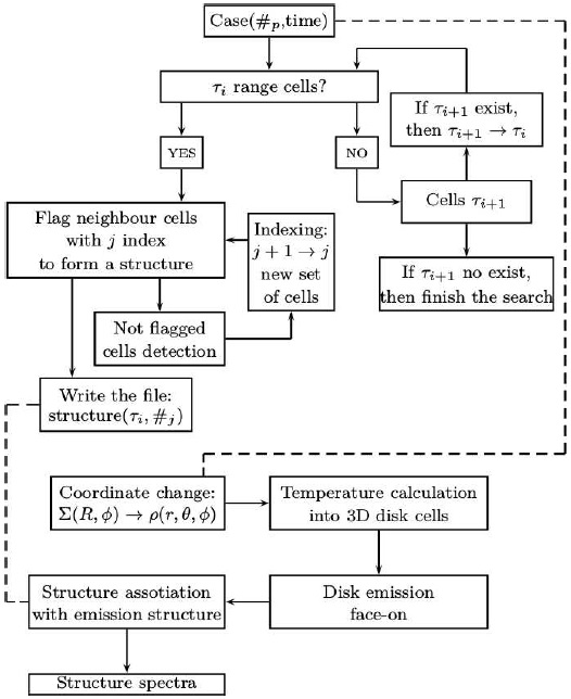
Once the dust optical depth is characterized, we proceed to find the structures in an iterative way. The following steps are used to find the structures associated to different ranges of optical depth (see Figure 1).
Case Selection. We choose a specific output ofthe hydrodynamical simulation.
Each hydrodynamical cell is identified with aflag as a member of an optically thin, intermediate or thick structure.
We analyse the neighbourhood of flagged cells.If a neighbour cell has the same range in τ then it will be flagged as a member of a structure.
We repeat Step 3 for all the contiguous cellsof the forming structure which share the same range in optical depth. Next we repeat the process for all the unflagged cells, for the three optical depth bins. This procedure form blocks of cells that we will name ‘the structures of the disk’.
We print the structures into individual files inorder to count them and look at properties like radial size and mass.
We notice that the structures found using this algorithm come from a simulation with an uniform alpha viscosity parameter. However, the new distribution of material (particularly the optically thick structures) has the effect of changing the physical conditions, which in some cases will reduce the heating rate. This will change the degree of ionization in these places and the magneto rotational instability (MRI) will define a non-homogeneous viscosity related to the created turbulence. This means that some of the structures formed (due to embedded planets) can become ‘dead zones’ (Martin et al. 2012) due to a reduced viscosity.
2.1.4. The Structure Spectrum
In order to get a spectrum (from the 2D simulations) for each structure identified by the algorithm described in § 2.1.3, we couple the algorithm with the Monte Carlo radiative transfer code RADMC-3D2( Dullemond in prep, which is based in RADMC-2D Dullemond & Dominik 2004). We proceed as follows:
1. We change cells with a surface density 2D to a volumetric density 3D. The conversion from surface density Σ(R,φ) in 2D polar coordinates to bulk density ρ(r,θ,φ) in spherical coordinates to be used by RADMC-3D is made by the following steps. First, we allocate the bulk density in the disk plane, i.e. θ = π/2, with the approximation
for the density above the midplane. Considering a vertically isothermal distribution the equation is
where h is the height scale and z = rcos(φ) is the disk height. The height scale is selfconsistent with the hydrodynamical simulations, i.e., h = 0.029(r/AU)1.25, which is required by the assumption of a vertically isothermal disk (see § 2.1.1).
2. We calculate the disk temperature by using aroutine in RADMC-3D.
3. We calculate the disk emission (face on, i.e.,0◦ inclination) in the line of sight for all wavelengths, and save it in a file as an array in the pixel space xy.
4.We associate the structures (previously found,described in § 2.1.3) in pixel space, in order to associate them with their respective spectra. A spectra association can be seen in Figure 6.
2.1.5. Estimate of the Mass Inside the Hill Radius
To estimate the mass inside the Hill Radius RH, we take the sum of the
masses m
ij of the cells with ij index in the planet neighbourhood such that
their mean position
The left part of the inequality is the distance between the cell position and the planet. The mean cell position is:
while the planet position is
Now using the condition given in equation 4, we calculate the grid areas inside the Hill Radii. After that, we can determine their mass contribution (see Figures 22-24) by optical depth range (according to § 2.1.2).
The left plot in Figure 2 shows the evolution of the semi-major axis (until 3.2 × 10⁵ yrs) of two planets, using three grid resolutions (Nφ,Nr) = (384,256), (384,384) and (448,384). In the right plot is presented a convergence check of the area inside the Hill Radius RH for these cases, with the evolution of the number of cells and the area. The number of cells inside the Hill radius is larger than 20, so the estimate of the dust mass is reasonable. Notice that the semi-major axis and area inside the Hill radius do not appreciably change when a better resolution is used. In particular, the area in this figure contains the dust mass shown in the top-left plot of Figure 22.
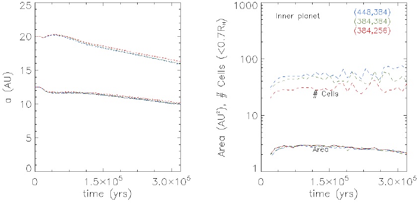
Fig. 2 Left: Semi-major axis evolution (until 3.2×10⁵ yrs) for several grid resolutions; (Nφ,Nr) = (384,256), (384,384) and (448,384), for low (red), intermediate (green) and high (blue) resolution, respectively. The upper (lower) curves represent the evolution of the outer (inner) planet. Right: Comparison between all the resolutions for the number of cells and the area, evolution of the grid area within 0.7RH of the interior planet, and the number of cells in the grid area by grid resolution. The color figure can be viewed online.
2.1.6. Hydrodynamical Model for Structures in V1247 Ori
We apply the method described in previous sections to analyze the disk structures of the stellar system V1247 Ori. Caballero & Solano (2008) found that this source is a member of the ǫ Cluster at a distance of 385 ± 15pc and with an age of 510 Myr. Originally it was thought to be an A5III star (Schild et al. 1971); recently it has been reclassified as a F0V star (Vieira et al. 2003; Kraus et al. 2013). Using the pre-main-sequence evolutionary tracks from Bressan et al. (2012, PARSEC release V1.0), Kraus et al. (2013) estimate the mass as M∗ = 1.86 ± 0.02 M⊙, and the age as t∗ = 7.4 ± 0.4Myr.
This object is particularly interesting and adequate for a study with our method because, besides a well sampled SED, there is evidence of asymmetric density structures inside the disk (Kraus et al. 2013). Combining interferometric and spectroscopic observations from NIR to MIR, they modeled the spectrum of the disk, which includes an optically thin gap in the range ≈ 0.3−44 AU. They found the closure phases measured by AMBER to be zero within the uncertainties of ∼ 5◦ (see their Figure 2), which is consistent with a centro-symmetric brightness distribution on scales < 30 mas (r < 12 AU). Additionally, using aperture masking observations in the H, K’, and L’ bands, they observed asymmetries in the brightness distribution on scales of ≈ 15 − 40 AU. They also found that the disk has an inclination angle around i = 31o, i.e., close to face-on.
In our model, we adopt the calculation of stellar mass and age, M∗ = 1.87 M⊙ and t∗ = 7.4 × 10⁶ yrs, by Kraus et al. (2013). We assume a distance to the source of 385pc (Terrell et al. 2007; Caballero 2008). We take parameters of the protoplanetary disk as follows: Mdisk = 0.02 M∗ (which is consistent with the mass from a typical classical T Tauri disk), and a radial range from 0.18 AU (Kraus et al. 2013) up to ≈ 500 AU (consistent with a source spectroscopically similar to the resolved disk WL16 (Beckford et al. 2008)). The surface density slope is set equal to one, i.e., Σ = 104(AU/r) g cm−2.
As our initial condition, we assume that the gap is already formed. A more
consistent scheme would imply that each planet starts as a small mass ‘seed’
which accretes matter and migrates in the disk until finally opening and
maintaining a well formed gap, as in the model of V1247 Ori by Kraus et al. (2013). However, the evolution
of the system is not predictable, and we would need to run a large number of
simulations in order to obtain a consistent model for V1247 Ori. We point out
that the parameters for the planetary system associated to the gap formation is
just one possible scenario for the interpretation of this object. We require
more detailed observations in order to constrain the embedded planetary system
and to break the innate degeneracy of the modeling. Here, our aim is to analyse
the structures in the gap. In order to make a self-consistent pretransitional
disk model, as an initial condition for the simulation we divide the total mass
of the disk as follows: the inner disk mass Mdisk,in, the outer disk
mass Mdisk,out, the mass in the gap Mgap, and the total
mass of the planets Mp,tot. The inner disk mass is
The total mass of all the planets is
The multiplanetary choice for V1247 Ori is motivated by studies by Johnson et al. (2007), which show a larger efficiency of planetary formation with increasing stellar mass. They found that low-mass K and M stars have a 1.8% ± 1% planet occurrence rate compared to 4.2% ± 0.7% for solar-mass stars and 8.9% ± 2.9% for the higher mass subgiants; V1247 Ori would belong to the last classification. In particular, subgiant stars in the mass range 1.7M⊙ < M < 1.95M⊙ have planets with masses from 0.53 to 25 MJ. We think that larger planets could be common around stars like-V1247 Ori.
We propose that a multiplanetary system is responsible for creating the asymmetries in the ≈ 40 AU gap of V1247 Ori. Actually, 22% of the detected planets belong to multiplanetary systems (see the database in exoplanets.eu). The initial gap has a size from 2 to 55 AU (where we choose this range in order to produce a relaxed optically thin gap from ≈ 2 to ≈ 45 AU, after 104 yrs). Seven mutually resonant (2:1) planets (from 2.6 to 41.9 AU) are required to cover the relaxed gap. Note that the observations of stars within the mass range, 1.7 M⊙ < M < 1.95 M⊙ show nine massive planets with semi-major axes α > 2.5 AU (see Table 1).
Table 1 Semi-major axis α > 2.5 AU and masses of planets hosted by stars with masses from 1.7 − 1.95M⊙
| Planet name | Semi-major axis [AU] | Mass [MJ] |
| HIP 97233 b | 2.55 | 20 |
| HD 4732 c | 4.6 | 2.37 |
| HD 145934 b | 4.6 | 2.28 |
| HD 154857 c | 5.36 | 2.58 |
| Beta Pic b | 13.18 | 7 |
| 51 Eri b | 14 | 7 |
| HIP 73990 b | 20 | 21 |
| HIP 73990 c | 32 | 22 |
| Fomalhaut b | 115 | 3 |
The table shows that Fomalhaut b (3 MJ) at 115 AU (detected by the image method and at a relatively short distance of 7.7 pc) indicates that planets could normally exist at larger radii. The nine planets in the table with semi-major axes a > 2.5AU only represent 23 % of the total. However, we argue that this depletion is due to observational bias against detection at larger radii, i.e., to the difficulty to find planets at large distances from the star by the most successful methods (radial velocity and transit). With this in mind, and noting the similar observed planetary frequency between the stellar mass ranges 1.72 and 1.76 M⊙, and between 1.90 and 1.91 M⊙ (similar observed planetary frequency in spite of the observational bias against planet detection at low stellar masses) we conclude that the planets in the radial range required for our model for V1247 Ori do exist in real cases. Although the formation process of multiplanet systems inside the gaps is uncertain, they have been discovered around Sun-like and late type stars: HD 10180 (seven planets, Lovis et al. 2011); HD 219134 (seven planets, Vogt et al. 2015); TRAPPIST-1 (seven planets, Gillon et al. 2017); Kepler-90 (seven planets, Schmitt et al. 2014); HD 40307 (six planets, Mayor et al. 2009; Tuomi et al. 2013); Kepler-20 (six planets, Gautier et al. 2012; Buchhave et al. 2016); Kepler11 (six planets, Lissauer et al. 2011). This motivated us to develop hydrodynamic simulations with several planets embedded in the protoplanetary disk model for V1247 Ori. However, these simulations are not enough to show how the planets can cover the whole semi-major axes range, because planetesimal bodies can induce inner (outer) migration. This issue is beyond our present goal.
Applying the conditions for the planet resonance and masses mentioned above, we found that there are seven planets in the gap. From the inner to the outer one, their positions and initial masses are: 2.6 AU, 0.2 MJ; 4.1 AU, 0.31 MJ; 6.6 AU, 0.40 MJ; 10.4 AU, 0.53 MJ; 16.6 AU, 0.65 MJ; 26.4 AU, 0.76 MJ; 41.9 AU, 0.85 MJ. The semi-major axes are fixed. The system is relaxed after the first 104 yrs. Afterwards, planetary accretion is allowed (with the prescription by Zhu et al. 2011 with an accretion parameter f=1)3. With a graphic card for computational advantage we ran the simulations with FARGO3D, in its 2D setup (to resemble the old version of FARGO). The hydrodynamical mesh only considered the radial scale from 1 to 100 AU, because we were interested in possible structure formation in the gap (with 256 radial and 256 azimuthal spaces, logarithmically and arithmetically distributed, respectively).
In order to analyse the modelled structures spectra of this source in a 3D environment, we extrapolated the height scale as h = 0.5r1.3, which is compatible with the models of HD 169142 in Osorio et al. (2014). Finally we used equations 1 and 2 to create the spectra with the RADMC-3D code. Complementary to the hydrodynamical simulations, we ran a static model in the radiative transfer code, with an optically thick inner and outer disk, and an optically thin gap.
3. RESULTS
In this Section we present the results for the simulations described in § 2. In particular, we show information relevant for the geometrical and physical characterization of the structures formed inside the gap shaped by the dynamical evolution of the immersed planetary system. A noteworthy fact is that the interaction between the gas and the planets implies that the latter change their orbital parameters.
3.1. The Set of Hydrodynamical Simulations
After the gap formation, the planetary system slowly migrates towards the star over a time longer than the viscous timescale. The gap is joined to the migrating planets. During the simulation, the eccentricity of the planets changes but not appreciably; this will be explained below. These effects will leave their imprints in the formation of structures; we take them into account in the included physics of the simulations. The planets are radially free to move due to torques with the disk material; the semi-major axes vary by a mean factor of 0.79/0.85/0.92 during the simulation (until 3.5 × 10⁵ yrs), for 2, 3 and 4 planets embedded in the disk, respectively. In the three cases the gap slowly migrates towards the star. For the other cases where f = 10 (until 4.5×10⁵ yrs) and f = 100 (until ×106 yrs), the semi-major axes vary by a mean factor of 0.62/0.8/0.93 and 0.5/0.75/0.9, respectively. Notice that at this stage of the simulations, only for the cases with f = 100 the cavity does not have an optically thin environment. For cases with a gap, the mean semi-major axis diminishes by a factor of 0.78. During the time span of the simulations, planet scattering is not produced. Over most of the simulation time all planets are trapped into 2:1 mutual resonances. During the clearing of the disk (a stage not included in this work) planet scattering could occur, resulting in the escape of some members of the planetary system. This work focuses on the stage with a disk; the evolution during the stage without a disk is beyond the scope of the paper. As in Zhu et al. (2011), we show that either a larger number of planets or a lower planetary accretion parameter imply a lower mean planetary migration. The largest value of the eccentricity is 0.3 (found for the 4-planet case with f = 1); the mean final eccentricity for the planets, taking into account all the simulations, is 0.17.
Figure 3 shows the stellar accretion rate for a configuration of 2, 3 and 4 planets and the accretion planetary parameter f = 1. We calculate a larger stellar mass accretion rate with a lower number of planets. Until 3 × 10⁵ yrs, the stellar accretion rate for a 2-planet system reaches a value of the order of 10−10 M⊙yr−1, while that of the 3- and 4-planet configurations is an order magnitude smaller. This is because a large number of planets restricts the material circulation from the outer to the inner disk through the gap between the planets.
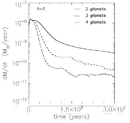
Fig. 3 Stellar mass accretion rate for 2, 3 and 4 planet configurations, which correspond to the solid curve, dashed and dash-dotted, respectively.
Figure 4 shows the mean azimuthal gas density for the two-planet case with f = 1 at evolutionary times 5×10⁴, 1×10⁵, 2×10⁵ and 3×10⁵ yrs; we use this example because the simulations show that the combination of a lower planetary accretion parameter and a lower number of planets produces a deeper gap. The density of the inner disk decreases by two orders of magnitude at 3 ×10⁵ yrs, while that of the gap region decreases by four orders of magnitude, and the external disk does not suffer any variation.
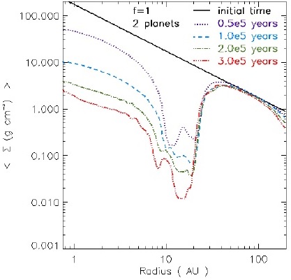
Fig. 4 Azimuthal mean gas density at times t = 0, 0.5 × 10⁵, 1.0 × 10⁵, 2.0 × 10⁵, and 3.0 × 10⁵ yrs, which correspond to the solid curve (black), dotted (purple), dashed (blue), dash-dotted (green), and dash-dot-dotdot (red), respectively, for an accretion planetary parameter f = 1, and 2 planets. A similar figure is shown in Zhu et al. (2011). The color figure can be viewed online.
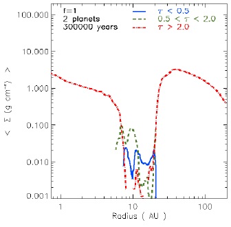
Figure 5 shows an example of the azimuthal mean surface density for the three ranges of optical depth considered: τ ≤ 0.5, 0.5 < τ < 2.0 and τ ≥ 2.0 corresponding to optically thin, intermediate and optically thick emission, respectively. In the case of two planets at 3×10⁵ yrs, we found that the gap density is dominated by optically thin and intermediate material, while only the material of the inner and outer disks is optically thick.
3.2. The Complex Structure Emission
In order to visualize the relation between the geometry of the structures and their spectra, Figure 6 shows, for the case of the two planets, the relation between the emission of complex structures in the disk and their contribution to the spectrum for a planetary accretion parameter equal to 1 at 3 × 10⁵ yrs. We show this case as a good example of a pre-transitional disk, which has an optically thick inner disk, a gap, an optically thick outer disk, an optically intermediate region that connects the two disks, and optically thick structures present inside the gap. The colors match the structures with their respective spectrum. We can see that the star plus the disks (inner and outer) dominate the spectrum. We found an optically intermediate structure with a maximum value in its SED of ≈ 10−11 ergcm−2 s−1, an optically thin structure with a maximum of ≈ 8 × 10⁻¹² ergcm−2 s−1, and two optically thin structures with a maximum of ≈ 10−13 erg cm−2 s−1. We will see in § 3.5 that these two optically thin structures have a dust mass of ≈ 10−4 M⊕; an optically thick structure with a slightly larger mass does not reach a maximum value of 10−13 erg cm−2 in its SED.
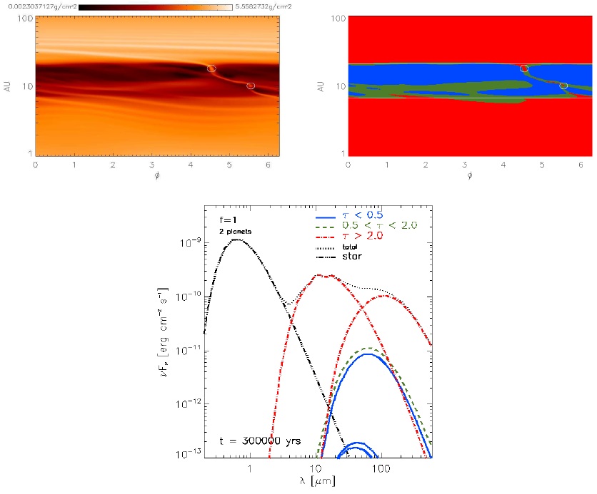
Fig. 6 Snapshot at 3 × 10⁵ yrs. Connection between the structures found in ranges of optical depths and their SEDs. Top Left: Density polar 2D map from 1 to 100 AU. Top Right: The 2D polar map where the structures are showed with their respective range of optical depth: optically thin (blue), intermediate (green) and thick (red) structures. Horizontal white lines show radii where the mean optical depth ⟨τ(r)⟩ = 2. The small closed lines shows the Hill radii of the planets. Bottom: Simulated SEDs with the target at 140 pc. The dotted curve (black) shows the total spectrum (structures + star). The optically thick inner (outer) disk dominates the spectrum. An optically intermediate structure and three optically thin ones have a maximum flux in SED of > 10−13 erg cm−2 s−1 The rest of the structures do not appear in the plot because their SEDs have a maximum flux < 10−13 erg cm−2 s−1. The solid curves (blue), dashed (green) and dash-dotted (red), correspond to structures optically thin, intermediate and thick, respectively. The color figure can be viewed online.
3.3. The Gap Filling Factor
The filling factor of a region is defined as the ratio between the optically thick area and the total area. This important geometric quantity allows us to understand the disk structure without the necessity of details. This quantity is commonly used by authors who desire to model protoplanetary disk spectra without the data from hydrodynamical simulations (Dodson-Robinson & Salyk 2011; Perez et al. 2014). Figure 7 shows a complex mean azimuthal radial filling factor for a planetary accretion parameter equal to 1, and 2 planets, at times 1, 2, 3×10⁵ yrs, top-left, top-right and bottom, respectively. At 105 yrs, the filling factor is dominated by optically intermediate regions; at 2×10⁵ yrs, by optically intermediate and thin regions; and at 3×10⁵ yrs, by optically thin regions. Some authors use a mean optically thick filling factor of the gap to adjust models to observed SEDs, e. g. Dodson-Robinson & Salyk (2011). They model the SEDs of GM Aur and DoAr 44, obtaining a good fit using a filling factor of 0.03 and 0.1, respectively. We have defined the gap from an inner to an outer radius such that there is material with τ ≤ 2, where τ = hΣiκ10µm. We can see that the mean optically thick filling factor hfgapi = Agap,τ>2/Agap decreases with time, starting with a value of 0.1 at 1×10⁵ yrs and finishing with a value of 0.01 at 3 × 10⁵ yrs.
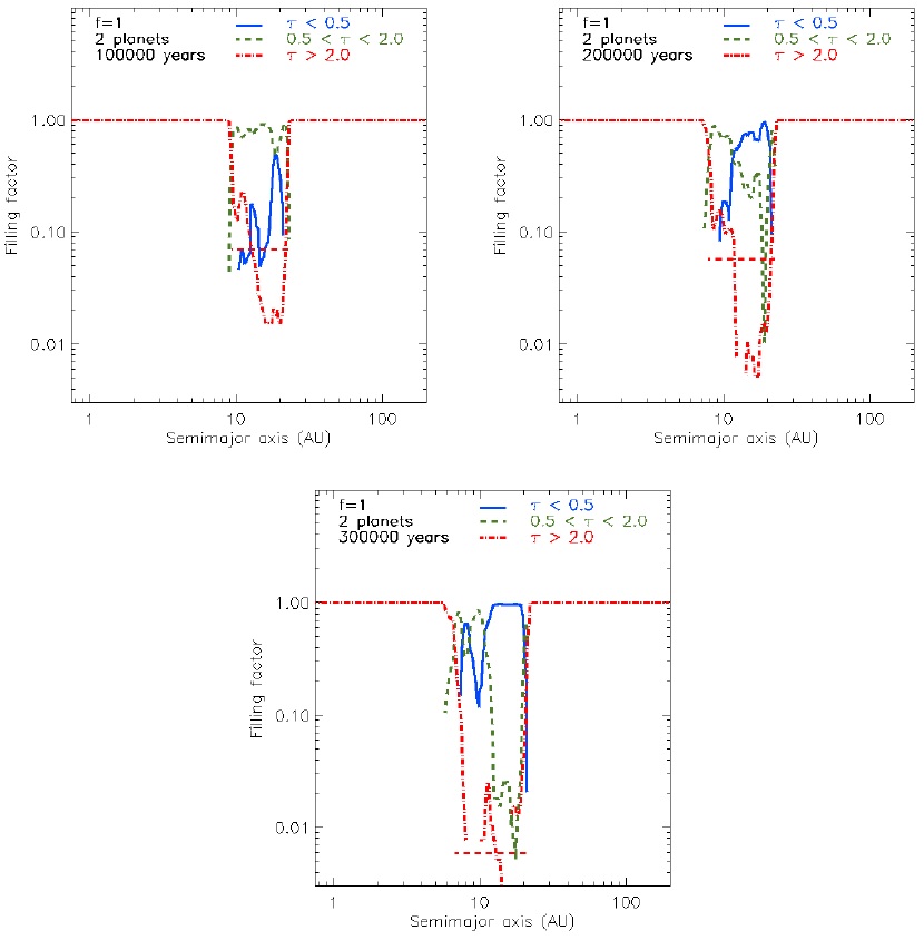
Fig. 7 The mean azimuthal filling factor by range of optical depth. The solid curves (blue), dashed (green) and dashdotted (red), correspond to optically thin, intermediate and thick regions, respectively. The dashed horizontal line in the gap region is the mean filling factor of optically thick material, where the gap is defined for any r with τ ≤ 2 such that τ = hΣ(r)iκ10µm. Top left: 1 × 10⁵ yrs. Top right: 2 × 10⁵ yrs. Bottom: 3 × 10⁵ yrs. The color figure can be viewed online.
3.4. The Size of the Structures
Once the structures are well characterized geometrically by cell blocks on the disk, we can obtain the inner and outer radial edge for each structure, so as to estimate their radial size. We obtain other quantities such as the mass and mean position of the structure, see § 3.5 and § 3.6, respectively.
Figure 8 shows the radial sizes of the structures in the ranges of optical depth considered for 2 planets, and a planetary accretion parameter equal to 1 at 3 × 10⁵ yrs. The lower and upper horizontal lines are the inner and outer borders of the gap, respectively. We note that the inner (outer) border is located at ≈ 3 RH (≈ 2 RH) from the location of the inner (outer) planet. This is approximately half of the interaction distance considered by DodsonRobinson & Salyk (2011), who found that a planet can open 4 to 5 RH gaps in ≈ 105 yrs. The same overlapping symbols (and colors) on this figure show very small structures. For the optically thick range (crosses): the first structure corresponds to the inner disk; the second one to the seven structures lying in the gap; finally the eighth structure begins inside the gap and finishes at the external border of the disk. For optically intermediate ranges (squares): the first structure lies across the gap; the second and third small structures are located in the inner gap border; the fourth and fifth small structures lay inside the gap; and finally the sixth and seventh small structures are located at the external gap border. For optically thin ranges (triangles): the first structure lies at the inner gap border; the second structure lies across the gap; the third structure is located at the inner gap border; the fourth and fifth structures lie inside the gap. For the other planetary configurations (with a larger number of planets), the general description of the size of the structures is similar, except for the small structures which are located in the surroundings of the gap center sharing the three optical depth regimes. A detailed description of the behavior of the planet position versus their neighbour structures is presented in § 3.6.
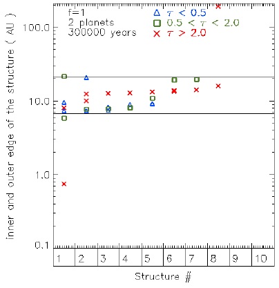
Fig. 8 Radial size of structures (at 3×10⁵ yrs), or inner and outer edge of the structure. The triangles (blue), squares (green) and crosses (red), correspond to the borders of optically thin, intermediate and thick structures, respectively. The inner (outer) symbols correspond to the inner (outer) borders. The solid top (bottom) horizontal line corresponds to the inner (outer) border of the cavity, rgap,in and rgap,out, respectively. i.e. where ⟨τ(r)⟩ = 2. The color figure can be viewed online.
For comparison, we note that when the indirect potential term is included in the hydrodynamic equations, the number of intermediate structures in the gap becomes larger than the number of optically thick structures without the inclusion of the indirect term. This happens because the external parts of the disk have a lower surface density, due to a slower migration rate, allowing a faster evolution of structures in the gap, i.e., the gap is easily cleared of optically thick structures, allowing the increase of the number of optically intermediate structures. Then, in terms of structure formation, the indirect terms do not have a significant influence on our structure analysis, just on the details. Note that including the terms, the gap occurs at a larger radius.
3.5. The Masses of the Structures
Figure 9 shows the contribution of the structures’ dust mass and optical depth range for a planetary accretion parameter equal to 1, and 2 planets, at 3 × 10⁵ yrs. Hereafter, we classify the structures as massive or non-massive. Massive structures are those for which the dust (gas) mass is above of 10−3M⊕ (0.1M⊕), while the non-massive structures are those having a mass below this value. The optically thick massive structure encompasses the innermost optically thick region which approximately defines the inner disk; the eighth optically thick structure defines the outer disk; the first optically intermediate structure crosses the gap; and finally an optically thin structure defines the gap. These massive structures have a maximum flux in their SED above νFν ∼ 10−13 erg cm−2 s−1. The non-massive structures have fluxes below this value.

Fig. 9 Dust mass distributed in structures (at 3×10⁵ yrs) of well mixed silicate dust, organics and troilite; within a size range of 0.005 − 0.15 µm. The triangles (blue), squares (green) and crosses (red), correspond to optically thin, intermediate and thick structures, respectively. For reference to Figure 13, the dotted horizontal line corresponds to 10−3 M⊕, which separates the massive from the non-massive structures. The color figure can be viewed online.
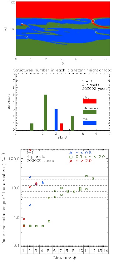
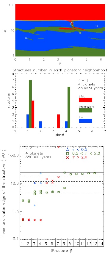
3.6. Structures in the Planetary Neighbourhood
The simulations contain an overwhelming amount of information. Here we present how the number of structures evolves in time in the neighbourhood of each planet; by neighbour structures we mean the ones around the mean semi-major axis of the planet. The neighbour structures affect the planetary accretion; a real description of this process is more complex than the picture presented here. Figures 10-12 present the number of structures around each planet, for the planetary system with four planets and a planetary accretion parameter f = 1, that corresponds to a scenario where the gap is easily and quickly formed. We should remember that the limits of the gap are such that ⟨τ(r)⟩ = 2 inside (outside) the inner (outer) planet. At 5 × 10⁴ yrs (Figure 10), small optically thin structures are starting to emerge in the neighbourhood of the inner planets; it is the start of the formation of the optically thin environment of the gap. At the same time, optically intermediate structures dominate the neighbourhood of the outer planets. At 2 × 10⁵ yrs (Figure 11), the optically thin structures merge to form a larger structure that eventually forms a gap dominated by optically thin material. An optically thick structure is located at the position of the third planet. At 3.5 × 10⁵ yrs (Figure 12) we find in the gap with an optically thin environment some optically intermediate structures related to the inner and outer planets, due to the transition to the optically thick region. Two optically thick structures in the neighbourhood of the third planet do not have the same spatial position as the planet, i.e., the optically thick structure is not necessarily physically linked to the planet. Thus, for each planet the distribution of structures is different, resulting in a planetary accretion that strongly depends on time and location of the planet. These results will be useful when high spatial resolution observations are available for the planetary neighbourhood. Also, we can see that the inner border of the gap evolves an order of magnitude faster (with a mean rate ≈ 1.4 × 10⁻⁵ AU yr−1) compared with the outer gap border (with a mean rate ≈ 3.7 × 10⁻⁶ AU yr−1). However, the mean migration rate of planets is ≈ 5.2 × 10⁻⁶ AU yr−1), i.e., faster than the outer gap border rate, but within the same order of magnitude. Thus, the outer gap border velocity could determine the mean planetary migration rate.
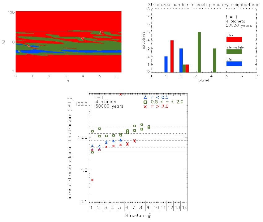
Fig. 10 Time evolution of the number of structures around each planet. The top left plot represents the polar 2D image of the optical depth for the hydrodynamical simulations at 5×10⁴ yrs. In the top right plot, the horizontal axis indicates the planet number: 1 for the inner and 4 for the outer planet. Each section is divided into 3, for thin, intermediate and thick structures, corresponding to blue, green and red colors, respectively. The vertical axis is the number of structures. The upper right, left and lower plots correspond to the system at 5 × 10⁴, 2 × 10⁵ and 3.5 × 10⁵ yrs., respectively. The bottom plot shows the correspondence with the radial size by structures (as shown in Figure 8). The horizontal dashed lines are the semimajor axis of the planets. The color figure can be viewed online.
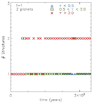
3.7. The Evolution of the Number of Massive Structures
In the snapshot of Figure 5 at 3 × 10⁵ yrs, we saw that the spectrum was dominated by two optically thick structures (the inner and outer disk). In order to detect the structures which dominate the disk spectra in each optical depth range, we define the massive structures as those more massive than 5 × 10⁻³ M⊕, which correspond to an optically thin structure in the same figure, with a maximum flux in the SED of νFν ≈ 8×10⁻¹² erg cm−2 s−1. Figure 13 shows the time evolution for the number of massive structures for 2 planets and a planetary accretion parameter equal to 1 until 3.5 × 10⁵ yrs. At 5 × 10⁴ yrs, the first optically intermediate structure arises in the disk. After that, at 7 × 10⁴ yrs, we can see the emergence of the inner and outer disk. Finally at 2 × 10⁵ yrs the optically thin structures arise in the gap, i.e., at this time the relevance of a hydrodynamical model for a pre-transitional disk begins. The non massive structures are not quantified because of their poor contribution to the total spectra. For instance, at 3 × 10⁵ yrs, the ratios of massive to non massive are 1:5, 1:6 and 2:6 for the optically thin, intermediate and thick ranges, respectively. A noteworthy fact is that the massive structures are few in number, so that they can be easily followed in time, for example, to describe the evolution of their emission.
3.8. Evolution of the SED for the Gap Structures
Figure 14 shows the evolution of the SED of a model with 2 planets and a planetary accretion parameter equal to 1. We can follow the SED evolution and the disappearance of the structures in the gap.
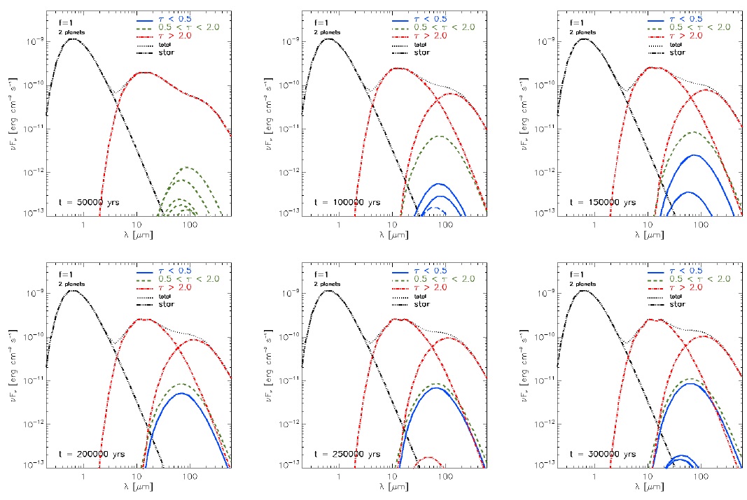
Fig. 14 Spectral energy distribution variation during the evolution. (i.e. for times 5 × 10⁴, 1.0 × 10⁵, 1.5 × 10⁵, 2.0 × 10⁵, 2.5 × 10⁵, and 3.0 × 10⁵ yrs). Shown are the spectra of the structures found above the horizontal line in Figure 9. The dotted curves (black) show the total spectra (structures + star). The solid curves (blue), dashed (green) and dash-dotted (red), correspond to optically thin, intermediate and thick structures, respectively. The color figure can be viewed online.
For example, at 5×10⁴ yrs, there are three optically intermediate structures, but only one remains at 1×10⁵ yrs. At this time the disk separates to form the inner and outer disk. From 2×10⁵ to 3×10⁵ yrs, in addition to the inner and outer disks, two massive optically thin and optically intermediate structures lie inside the gap. Both structures increase their emission contribution as the time increases: from 5 × 10⁻¹² to 8 × 10⁻¹² erg cm−2 s−1 for the optical thin structure, and from 8 × 10⁻¹² to 1 × 10⁻¹¹ erg cm−2 s−1 for the optical intermediate structure. However, as we will see in § 3.11, at these times the filling factor for optically thin structures is increased in the gap, while that for the optically intermediate is decreased. This will be discussed below.
3.9. The SEDs of the Structures while Varying the Number of Planets
Figure 15 (top) shows an increase in the number of structures as the number of planets increases for f = 1, at 3×10⁵ yrs. In the cases with two and three planets, the disk was separated mainly by two optically thick disks, which dominate the contribution to the spectrum. In the case with four planets, an optically intermediate structure can be seen in the range 10 − 50 µm, i.e., in the range including the silicate bands. This optically intermediate structure is the largest contributor to the SED surpassing the inner and outer disk contribution. In particular, the peak at 20 µm is produced by this structure. If the number of planets increases, the optically thin emission is the dominant one in the silicate bands. This result is reasonable because a greater number of planets manages to open a larger cavity. Note that Espaillat et al. (2010) required the emission of optically thin material in the gap to explain the silicate bands in the SED. We note in this example of a pre-transitional disk that the slope of the SED from 10 to 100 µm is negative; that means that there exist optically intermediate structures in the gap within an optically thin environment. Figure 15 (bottom) shows cases with a smaller planetary accretion (f = 10) for 2, 3 and 4 planets. The simulation time is not large enough for the disk to be separated in two parts. However, an increment in the number of structures as the number of planets increases is observed, but their contribution to the spectrum is negligible.
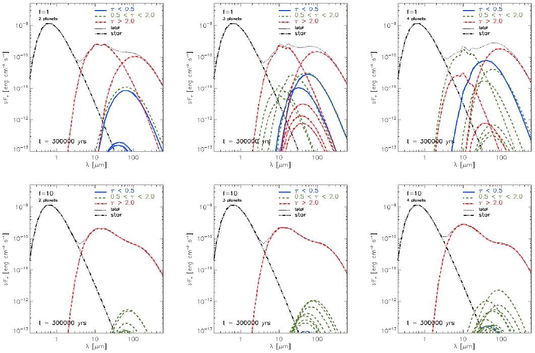
Fig. 15 The SED behaviour for two planetary accretion parameters (f = 1, top; f = 10, buttom). The dotted curves (black) show the total spectra (structures + star). The solid curves (blue), dashed (green) and dash-dotted (red), correspond to optically thin, intermediate and thick structures, respectively. The color figure can be viewed online.
3.10. The Gap Mass Evolution
Figures 16-18 show the mass evolution (in earth mass units, M⊕), of small dust grains (size range: 0.005-0.25 µm) in the gap for the three ranges of optical depth here studied. We consider that the gap mass is between the boundaries defined by the mean optical depth equal to 2, i.e. hτ(r)i = 2 = hΣ(r)iκ10µm. This happens at radii rgap,in = r < rp,in and rgap,out = r > rp,out, where rp,in (rp,out) is the semi-major axis of the inner (outer) planet. At the initial time, the mass between rp,in and rp,out is increased if the number of planets also increases. Hereafter, this mass will be referred to as the initial mass.
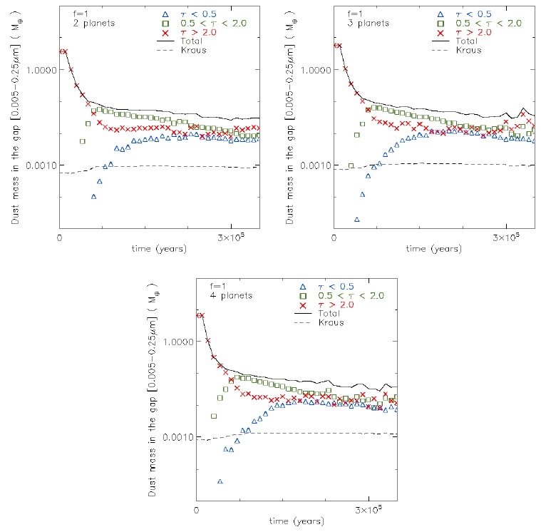
Fig. 16 The dust mass evolution in the gap (in earth mass units M⊕), for dust grains in the size range 0.005−0.25 µm, considering a MNR size distribution. The cases with 2, 3 and 4 planets and the smallest accretion parameter (f = 1), are ordered from top-left, top-right and bottom, respectively. The triangles (blue), squares (green) and crosses (red), correspond to the optically thin, intermediate and thick cases, respectively. The solid curve corresponds to the total dust mass. For reference, we show the model of Kraus et al. (2013) of the mass within the gap, dashed curve (with a surface density in the cavity of Σgap,Kraus = 9 × 10⁻⁶ gcm−2, see details in the § 3.10). The color figure can be viewed online.
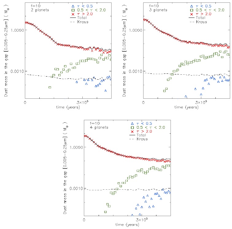
Fig. 17 Same as Figure 16, but with middle accretion parameter (f = 10). The color figure can be viewed online.
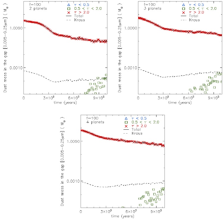
Fig. 18 Same as Figure 16, but with the largest accretion parameter (f = 100). The color figure can be viewed online.
Along the evolution of the gap mass for our set of simulations, we plot the optically thin gap mass of the V1247 Ori model of Kraus et al. (2013). It is shown by the dashed curves in Figures 16-18. This mass is defined as Mgap,Kraus = Σgap,Kraus ×π(rgap,out 2 −rgap,in 2), with Σgap,Kraus = 9×10⁻⁶ gcm−2, where the last value is the best fit to their V1247 Ori spectral model, in which they only include carbon dust grains. However, this value is smaller by a factor of 0.72 than the value we found in our model in § 3.13.
The case with 2 planets and planetary accretion parameter f = 1 (top-left in Figure 16) at 8 × 10⁴ yrs (in which the disk has separated into an inner and an outer disk, see Figure 13), shows that the gap total mass (the solid curve in the Figure 16) has been reduced by almost two orders of magnitude from its initial value. At this time, the mass of the gap is dominated by optically intermediate material. We note that the mass of the optically thin material in the gap is Mgap,Kraus. After 2×10⁵ yrs, the material for each optical depth range has a comparable mass. However as we see in Figure 19, the filling factor between material in the gap for the ranges of optical depth is not directly related to the mass contained in the gap. For the cases of 3 (top-right in Figure 16) and 4 (bottom in Figure 16) planets, the gap opening effects are faster than in the case of 2 planets.
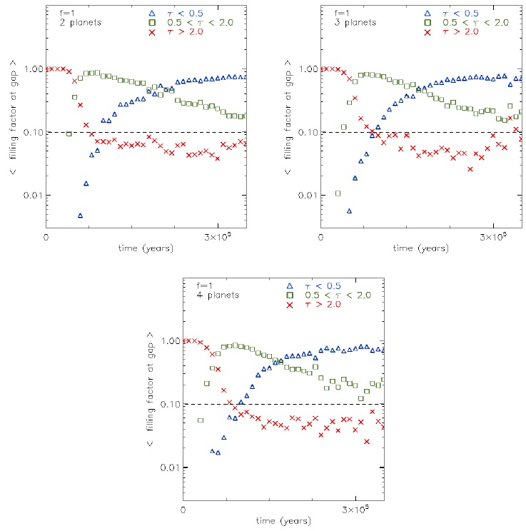
Fig. 19 Mean filling factor evolution in the gap. The triangles (blue), squares (green) and crosses (red), correspond to optically thin, intermediate and thick structures, respectively. For comparison, the horizontal dashed line shows the value to produce the best fit for the pre-transitional disk DoAr 44 deduced by Dodson-Robinson & Salyk (2011) (see their Figure 5). The color figure can be viewed online.
The case with 2 planets and f = 10 (top-left in Figure 17) at ≈ 4 × 10⁵ yrs shows that the mass of the optically intermediate structures is equal to the mass of the optically thick structures. The cases for 3 and 4 planets (top-right and bottom in Figure 17, respectively) do not show the same behaviour. This happens because the planetary accretion is faster in the case with 2 planets than in the cases with 3 and 4 planets, so that the gap structures in the latter cases become optically thicker. Around 9 × 10⁵ yrs in the case with 2 planets, the optically thin Kraus mass Mgap,Kraus is equal to the mass of the optically thin material detected in our hydrodynamic simulations. However, the gap mass of the optically thick and intermediate structures dominates over the optically thin structures. This is important because a lot of material is located in non-optically thin structures, and hence most of the material is inside structures not considered in the model of V1247 Ori by Kraus et al. (2013).
The cases with f = 100 (Figure 18), analysed for 106 yrs, do not show optically thin structures. However we observe the appearance of optically interme diate structures at 7 × 10⁵, 6 × 10⁵ and 5 × 10⁵ yrs, when considering 2, 3 and 4 planets, respectively. The presence of intermediate structures depends on the gap size which in turn depends on the number of planets.
The main results of our analysis are: (1) a larger number of planets generates a larger mass of the gap; (2) like in Zhu et al. (2011), a larger planetary accretion parameter corresponds to a larger mass of the gap (notice that a larger planetary accretion parameter means smaller accretion by the planets).
3.11. The Evolution of the Filling Factor of the Gap
Figure 19 shows the evolution of the mean filling factor of the gap. The cases with 2 (top-left), 3 (top-right) and 4 (bottom) planets and f = 1 are shown here. As an horizontal dashed line we display the filling factor of the gap region obtained by Dodson-Robinson & Salyk (2011) in their model of the spectrum of DoAr 44. They found that the best fit required a filament of optically thick material with filling factor equal to 0.1.
The case with 2 planets shows the stage when the gap is dominated by optically intermediate material, from 5 × 10⁴ yrs to 2 × 10⁵ yrs, and the stage of the gap dominated by optically thin material starting at 2 × 10⁵ yrs.
At 3 × 10⁵ yrs, with the gap dominated by optically thin material, the filling factor of the optically thin, intermediate and thick regions is approximately 0.7, 0.25 and 0.05, respectively, i.e., there is an order of magnitude difference between the filling factor of optically thin and thick material. At the same time, we observe in Figure 16 that the gap mass of optically thin and thick material has comparable values, ≈ 10−2 M⊕. A similar behaviour is observed in the gap for the cases with 3 and 4 planets, but the dominance of the filling factor by optically thin material occurs later than in the case with 2 planets.
For the case of 2 planets, this is consistent with results shown in Figures 6 and 9, where the small optically thick structures in the gap contribute to the mass, but have a small contribution to the spectrum (a difference of at least two orders of magnitude between optically thin and thick structures in the gap, ≈ 8×10⁻¹² and < 10−13 erg cm−2 s−1, with masses ≈ 5 × 10⁻³ and ≈ 2 × 10⁻⁴ M⊕, respectively. We could increase the mass of the optically thick structures by an order of magnitude compared to the mass of the optically thin structures, and the latter would continue to dominate the spectrum. This means that optically thick regions could hide one order of magnitude more material than optically thin structures. The optically intermediate structures can only hide twice the mass of the optically thin structures. This fact becomes relevant when fitting the gap spectrum with optically thin material. In other words, a fit with only optically thin material clearly underestimates the amount of material in the gap.
We notice that at ≈ 8 × 10⁴ yrs the filling factor for the case of 2 planets is equal to the filling factor of the gap region of DoAr 44. At the same time, the optically intermediate material has a filling factor of 0.85. This is the reason why the study of emission of structures in several optical depth ranges is important, in order to estimate the amount of material hidden by these structures.
Figure 20 shows the evolution of the mean filling factor of the gap for the cases with 2 (top-left), 3 (top-right) and 4 (bottom) planets and f = 10. The stage when the gap is dominated by optically intermediate material starts at 3.5 × 10⁵ yrs. For 3 and 4 planets, the optically thick material always dominates the filling factor of the gap until the end of the simulation, at 4.5 × 10⁵ yrs.
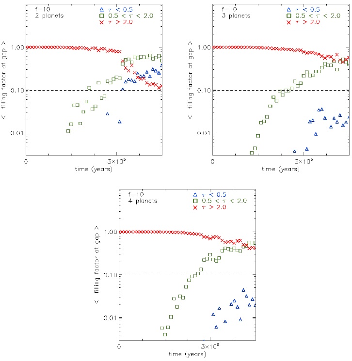
Fig. 20 Same as Figure 19, but with middle value for the accretion parameter. The color figure can be viewed online.
Figure 21 shows the cases with 2 (top-left), 3 (top-right) and 4 (bottom) planets, and f = 100, at 106 yrs of simulation time. At this time the optically thick material dominates. Some optically intermediate structures appear at 8 × 10⁵ yrs.
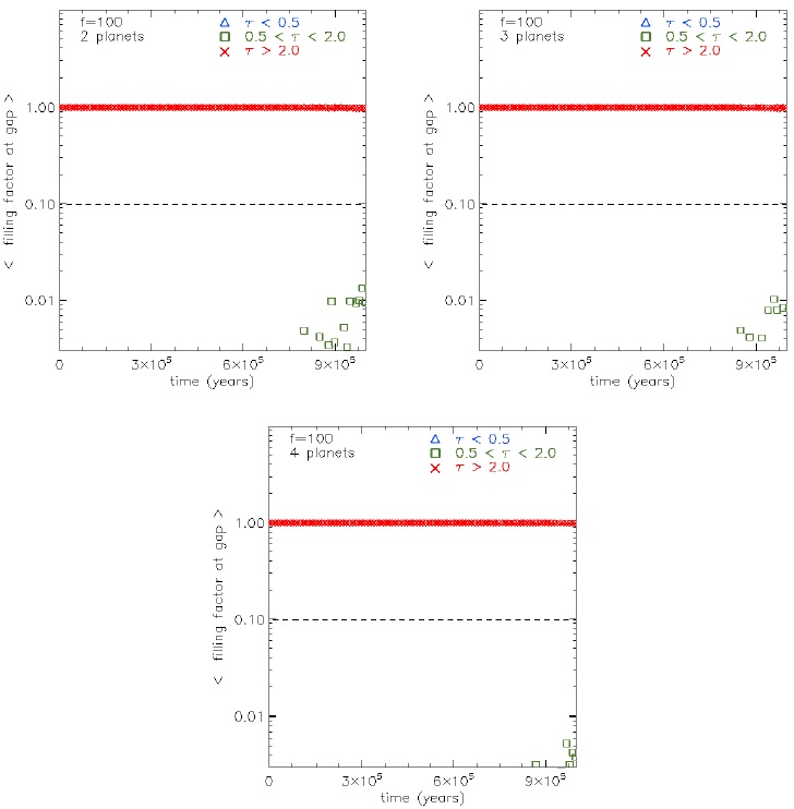
Fig. 21 Same as Figure 19, but with the largest accretion parameter. The color figure can be viewed online.
Summarizing, at times greater than 3 × 10⁵ yrs, our main results are: for f = 10, the optically intermediate and optically thin material predominate when the number of planets is small; for f = 1, the optically intermediate material eventually becomes dominant; for f = 100, the optically thick material is always dominant. It is important to note that the estimated mass (or filling factor) in the gap strongly depends on the evolutionary state of the system. This should be taken into account when modelling a particular system.
3.12. Evolution of the Dust Mass into the Hill Radius for the Innermost Planet
The description of the inner planet neighbourhood is highly important, because it lets us know whether it is possible to form satellites in the neighbourhood of the massive planets.
Figures 22 to 24 show the evolution of the dust mass within 0.7 Hill radius for the innermost planet in lunar mass units ML (1ML = 7.3477 × 1025 g) for the set of simulations developed in this work. We choose the 0.7 fraction of the Hill radius because all cells are completely contained inside the Hill radius; thus, this gives us a reasonable estimate of the mass inside this region (see § 2.1.5). We note that this is a rough analysis, because we do not include a detailed model for the physics present in the gas near the planet. For a better analysis, we should use an approach based on nested cells as in Ayliffe & Bate (2009) and Machida et al. (2008). However, this exercise could be useful to establish a better initial conditions for circumplanetary disks simulations with higher resolution.
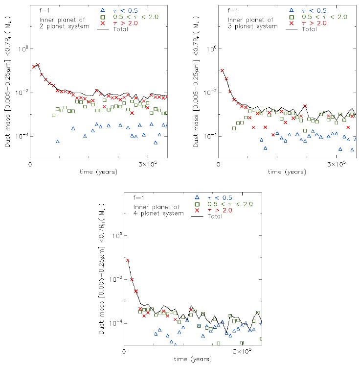
Fig. 22 Dust mass inside the Hill Radii for the inner planet of the corresponding system. The triangles (blue), squares (green) and crosses (red), correspond to optically thin, intermediate and thick cases, respectively. The color figure can be viewed online.
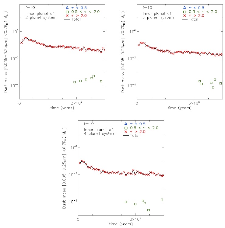
Fig. 23 Same as Figure 22 but with the middle accretion parameter. The color figure can be viewed online.
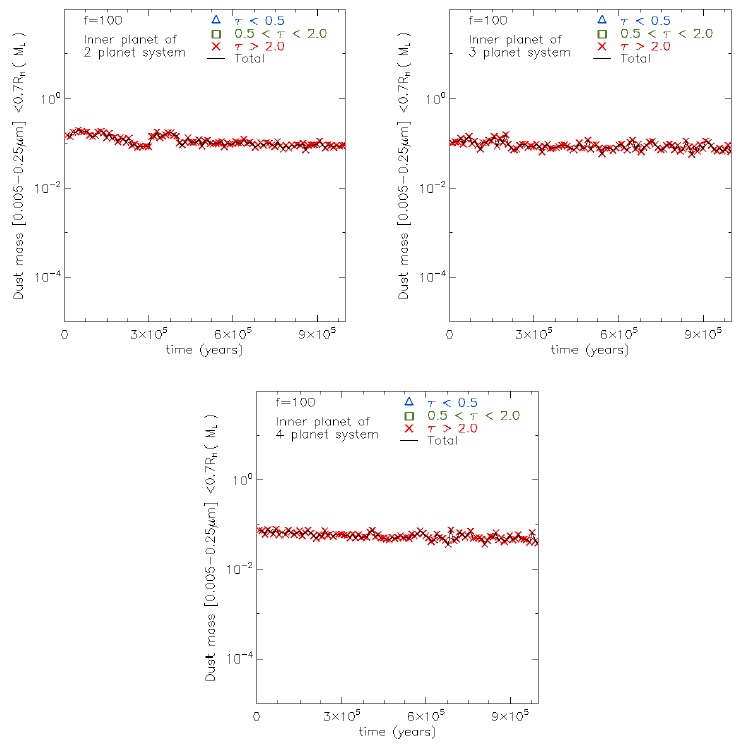
Fig. 24 Same as Figure 22 but with the largest accretion parameter. The color figure can be viewed online.
In simulations with f = 1 (Figure 22) and a simulation time of 3.5×10⁵ yrs, the mass within the Hill radius decreases from an initial value (10−1 ML) to 10−2, 10−3 and 10−4 ML for the 2, 3 and 4 planet cases, respectively. In the case with 2 planets, the mass of the optically thick dust dominates over that of the optical intermediate and thin ranges. In the case with 3 planets, the mass of the optically thick and intermediate dust dominates over the optical thin mass. Finally, in the case with 4 planets, the mass of the optically intermediate dust dominates over the optically thin mass. Summarizing, in all planet cases with f = 1, is clear that an increase in the number of planets allows a faster evolution of the structures in the different ranges of optical depth inside the Hill radius for the inner planets.
In cases with f = 10 (Figure 23), where the simulation time reaches 4.5 × 10⁵ yrs, the mass within the Hill radius decreases an order of magnitude, from 10−1 ML to 10−2 ML. We found that the mass present is slightly smaller with increasing planet number.
In simulations with f = 100 (Figure 24), at 106 yrs, we do not observe a significant decrease of the mass within the Hill radius.
A preliminary conclusion is that there is enough material (with a nearly constant rate in each case) to form the circumplanetary disk. Now, if we consider (like Dodson-Robinson & Salyk 2011) that 20% of the dust is visible in the range from 0.005 to 0.25µm, and the other 80% above millimetric size could become rocks and planetesimal bodies, then the values of mass within the Hill radius must be multiplied by 5. The details of moon formation are beyond the scope of this work.
3.13. The V1247 Ori Case
In this section we present non hydrodynamic and hydrodynamic models for the stellar system V1247 Ori; the latter are consistent with interferometric and photometric observations by Kraus et al. (2013). In both cases, we find a good fit to the observed spectrum. The non-hydrodynamic case consists of axisymmetric density structures; hence, the asymmetries found by the interferometric observations (Kraus et al. 2013) cannot be explained by this model. We present both cases as examples of how new observational information is required to find a system configuration closer to the reality.
3.13.1. Non-Hydrodynamic Case
Figure 25 shows a modelled SED of V1247 Ori; here we consider only amorphous carbon for the chemical composition of the disk, to make a comparison to the model by Kraus et al.. In order to extract the emission contributions by the optically thin and thick regions, we separate the model by structures, i.e., we consider the inner and outer disks as individual structures, and the gap as an optically thin structure. We produce the fit of the spectrum of the axisimmetric model, considering an optically thick inner disk (0.16-0.26 AU), followed by an optically thin gap (0.26-45 AU), and an optically thick outer disk (45-120 AU), where the inner and outer disks have optically thick material with a surface density profile of slope −1. These spatial ranges for the inner and outer disks are consistent with the model by Kraus et al., but we extended to 120 AU the size of the outer disk to explain the observed emission at longer wavelengths. The gap is an optically thin region with a constant density 1.25 × 10⁻⁵ gcm−2, which is denser by a factor of 1.38 than the gap proposed by Kraus et al. (2013). Contrary to the Kraus et al. model, the gap dominates the spectrum from NIR to MIR over the inner disk. To explain the difference between the two models we need to consider the thickness of the disk, which is required in the 3D radiative transfer code, in which the photons of the region can interact and escape from a thicker gap.
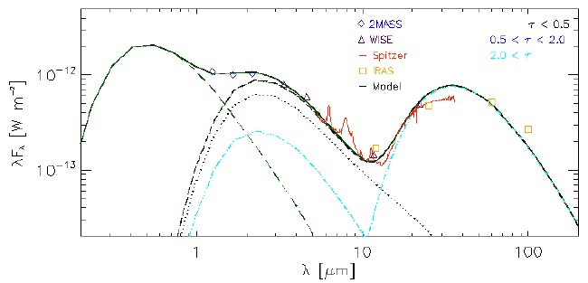
Fig. 25 Model for the spectral energy distribution of V1247 Ori, representing each region defined by ranges of optical depth for a static density profile. The dotted curve (black) is the spectrum of optically thin gap material; the dot-dashed curves (light blue) are the spectra of the optically thick inner and outer disks; the dashed curve (black) is the total disk contribution; the solid curve (black) is the total spectrum (disk + star). For comparison, we show the observed data (taken from their respective data base): 2MASS, diamonds (in blue); WISE, triangles (in brown); Spitzer, solid line (in red); IRAS, the squares (in yellow). The color figure can be viewed online.
3.13.2. Hydrodynamic Case
We start with a pre-formed gap, where seven planets have been embedded and fixed at different positions in the disk (see details of the initial model in § 2.1.6). Our hydrodynamic simulation is run until a time 3×10⁴ yrs is reached. The system relaxes during the first 1×10⁴ yrs. After this time, planetary accretion is allowed.
In the top panel of Figure 26 we show the evolution of the azimuthal mean density surface, at 1 × 10⁴, 2 × 10⁴ and 3 × 10⁴ yrs. The initial inner and outer steep edges of the gap have been smoothed at 1 × 10⁴ yrs. At 3 × 10⁴ yrs, the surface density of the inner disk reaches a value two orders of magnitude smaller than the initial value. The mass fraction of the planets (from inside out) has increased to 0.26, 0.22, 0.34, 0.52, 0.94, 1.78 and 5.05 compared to to their initial values. It follows that the outer planets are accreting more mass. This mass is coming from the outer disk.
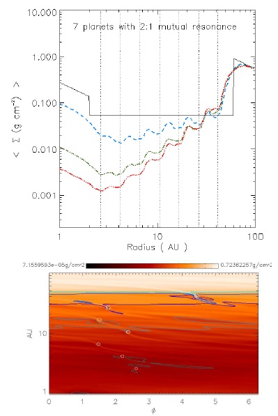
Fig. 26 Top: Mean azimuthal gas density with a preformed gap at initial time t = 0, and after 1.0 × 10⁴, 2.0 × 10⁴, and 3.0 × 10⁴ yrs of hydrodynamical simulation, which correspond to the solid (black), dashed (blue), dash-dotted (green), and dash-dot-dot-dot (red) curves, respectively. The seven initial locations of the 2:1 mutually resonant planets are shown as vertical dotted lines at their correspondent semi-major axis location. Bottom: Snapshot of surface density in g cm−2 at 3.0 × 10⁴ yrs, with a logarithmic scale color. The planet positions are well identified by their Hill radii. The optical depth isocontours: 0.01 (dark gray), 0.1 (neutral gray), 0.5 (blue), and 1.0 (azure), and 2.0 (cyan) are overplotted. The color figure can be viewed online.
Moreover, the first inner planet accretes more mass than the second one because it is closer to the inner disk. In the neighbourhood of each planet (inside the Hill Radii), we find the maximum accretion rate, which is equal to 10−13 M⊙ yr−1 for the first and second planet, 10−12 M⊙ yr−1 for the third and fourth planet, 10−11 M⊙ yr−1 for the fifth and sixth planet, 10−10 M⊙ yr−1 for the seventh planet.
In the bottom panel of Figure 26 we show a snapshot of the density map in polar coordinates (in a logarithmic color scale) and optical depth isocontours (τ = 10−2,10−1,0.5,1,2) at 3×10⁴ yrs, assuming the dust properties of § 2.1.2. Our optically intermediate region is defined between τ = 0.5 and τ = 2. Two external planets (specified by their Hill radii) are immersed in the optically intermediate region. We find the gap (the zone with optical depth τ < 2) within the region < 46 AU, similar to the region described in Kraus et al. (2013).
Figure 27 shows the size and mass of each structure for the two sub-ranges of optical depth, the 0.5 < τ < 1 and 1 < τ < 2 (in the optically intermediate range), and τ > 2 (the outer disk). Two asymmetric structures are found for each sub-range (see the left plot in the figure). These structures are located between ≈ 20 and ≈ 46 AU, as predicted by Kraus et al. (2013), where they propose asymmetric structures between ≈ 15 and ≈ 40 AU. This means that with our multiplanetary model, the asymmetric structures can be reproduced by two resonant massive planets. The masses predicted by these structures are around ≈ 10−5−10−2 M⊕ (see the left plot in the figure).
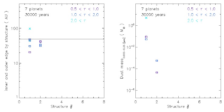
Fig. 27 Optically intermediate structures in the gap, and in the optically thick outer disk, after 3 × 10⁴ yrs. We show two ranges: the optically intermediate: 0.5 < τ < 1 (blue), and thick: 1 < τ < 2 (azure). The outer disk has τ > 2 (cyan). Like in Figure 8, the squares and crosses correspond to the borders of optically intermediate and thick structures. Left: Radial size of the structure, or inner and outer edge of the structure. Inner (outer) symbol of each, structure corresponds to inner (outer) border. The solid top horizontal line corresponds to the outer border of the cavity rgap,out, where ⟨τ(r)⟩ = 2. Right: Dust mass distributed in structures of well mixed silicate dust, organics and troilite; within a size range of 0.005 − 0.15 µm. The color figure can be viewed online.
Figure 28 shows the total modelled spectrum of V1247 Ori, the spectrum of each structure and the observed spectrum composed by data of several telescopes. The total modelled spectrum with a radial range between 0.16 AU and 110 AU, is obtained with the hydrodynamically simulated region (from 1 AU to 100 AU) and two non simulated regions (the inner region from 0.16 to 1 AU, and the outer region from 100 AU to 110 AU). We need an optically thick inner disk from 0.16 AU to 0.22 AU (with a surface density profile of slope −1) to model the spectrum of the inner region. We extrapolate the density in the radial range between 0.22 AU and 1 AU (100 AU and 110 AU) based on the simulation values of the density and a mean surface density profile slope at 1 AU (100 AU). The emission of the gap region (from 0.22 AU to ≈ 46 AU) dominates from NIR to part of the MIR. Particularly, it dominates over the emission of the optically thick inner disk. At longer wavelengths the emission of the optically thick outer disk (≳ 46 AU) dominates over the emission of the two optically intermediate structures of the gap. These two optically intermediate structures are the most massive ones of the gap (≈ 10−2 M⊕), and are located between 20 and 46 AU as seen in Figure 27.
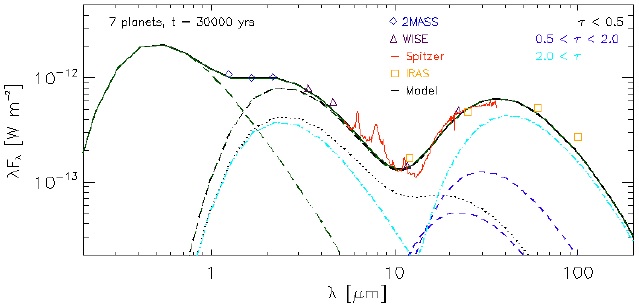
Fig. 28 SED model after 3 × 10⁴ yrs of the simulation, with the same observational data of Figure 25. The solid black curve is the total modelled emission. The contributions of the optically thin, intermediate and thick structures correspond to the dotted (black), dashed (blue) and dashed-dotted (cyan) curves, respectively. The dashed line (green) shows the result of the model for the stellar emission. The color figure can be viewed online.
4. DISCUSSION
The structures analysed in this work are completely defined by the hydrodynamical interaction of the disk gas with itself and the gravitational interaction of the planets with the gas in the disk. These interactions allow the formation of concentrations of matter in the disk that we call structures. However, there are other origins for the structures, which could be related to planet-disk interactions.
Alternative explanations for the formation of structures formation are:
Dust filtration: this is a physical mechanism where large grains are decoupled of the gas due to the drag forces; then the large grains are preferentially accumulated in a local maximum of density such as the gap edge formed by massive planet inmersed in the disk. Small grains can pass through the gap edge, and then they migrate towards the star. Thus, the larger grains are able to open a dust gap in the disk, and the smaller grains remain distributed throughout the disk (Paardekooper et al. 2006; Zhu et al. 2012). The difference between the small and large grain space distribution means that the dust opacity will not be homogeneous. This mechanism is supported by polarimetric observations of high resolution made by Garufi et al. (2013), which show a different spatial distribution for the small and large grains in protoplanetary disks. In the context of this work, this effect modifies the boundaries between optically thick, thin or intermediate regions. This slightly changes the number, mass and size of the structures, because the opacity changes occur in these transition zones between the structures. Thus, the distribution of dust in the structures could vary in the details but the qualitative picture should remain the same. In a future work, we are planning to include dust dragging in the analysis of structures for the long-term simulations (Alvarez-Meraz et’ al. in prep.).
Dead zones: these are regions where the magnetorotational instability (MRI) does not operate (Gammie 1996); this MRI mechanism defines a viscosity related to the turbulence created (Balbus & Hawley 1998). These zones are located at intermediate places: between an inner zone, where the MRI is activated by the high temperature (T > 103 K) which ionizes the alkali metals, and an outer zone, where the nonthermal source of the disk ionization (meanly by cosmic rays) is relevant. The importance of the MRI depends on the degree of ionization, which in turn depends on the efficiency of the heating mechanisms. Gammie (1996) show that such intermediate places (where the angular momenta transport by turbulence is not effective) have a surface density P > 100grcm−2. Such dense zones are not found in the viscosity models of this work.
Anticyclonic vortexes: they are produced with or without any planets. Structures formed without planets are produced by the Rossby wave instability (RWI); Lovelace et al. (1999); Regaly et al. (2012). These structures have been found in steep gas-pressure gradients of outer border of dead zones (Varniére & Tagger 2006; Terquem 2008). Planets can produce steep gas-pressure gradients resulting in anticyclonic vortexes (e.g., Lin & Papaloizou (2010), Zhu et al. (2014), Zhu & Stone (2014)).
The multiplanetary model for V1247 Ori is an ad hoc model, because of the large gap and the nonaxisimmetric structures between ≈ 15 and ≈ 40 AU (Kraus et al. 2013). However, the degeneracy of the model allows to fit the SED up to 20 µm, i.e. including the mid-IR, which is sensitive to the gap region. Better models for this source will require disk dispersion by photoevaporation, which results in a model with a smaller number of planets to explain such observed structures. To explain the extended outer disk (to ≈ 300 AU) with an arc emision at 108 ± 35 AU (Ohta et al. 2016) the model will require a perturbing planet farther away than the outer planet of the model of this paper (Alvarez-Meraz et´ al. in prep.). The new modelling should take into account the region outside the gap, but will not alter the modelling presented here, which is mainly focused on the MRI emission.
5. CONCLUSIONS
We summarize our conclusions as follows.
We develop a method to analyse the dust structures of proto.planetary disks at several ranges of optical depth, using hydrodynamical simulations. The method is able to detect structures as small as a hydrodynamical cell. Structures within the gap are well identified. We can know whether they grow or are fragmented into other structures. We also estimate the SED of these structures, which allows us to answer the question: how much material is hidden in optically thick or intermediate structures in the gap?. The optically thick and intermediate structures could hide mass an order of magnitude larger and twice the mass respectively, compared to to optically thin structures.
The structure analysis shows an increase in thenumber of structures as the number of planets increases. Also, we find a larger time scale for the formation of optically thin structures with a small accretion parameter. This is important, for instance, when the interpretation of observations requires some asymmetry in the system.
An analysis of the Hill radii scales shows that anincrease in the number of planets allows a faster evolution of the structures of different ranges of optical depth inside the Hill radii of the inner planets. This is a reasonable behaviour, because the material influx from the outer to the inner regions is limited by the planetary mass accretion and the number of planets. This means that the inner planets, in a planetary system, have a lower inflow of material compared to to the outer ones. This limits the amount of material that could arrive to the circumplanetary disks of the inner planets. For sure, this will change the initial condition for moon formation (Canup & Ward 2006). Thus, we speculate that there is a difference between the masses of moon systems of the inner and outer planets. However, this requires further analysis, and it is part of future work.
The hydrodynamical simulations presented in§ 2.1.1 consider planetary migration towards the central star, which allows the gap containing the planets to move towards the star. The mean final semi-major axis of the planetary orbits in the simulations changes by a factor of 0.78. However the mean migration rate of the optically thick outer gap border is smaller than the mean migration rate of the planets, but of the same order of magnitude. This means that the gap location does not change appreciably during the simulation. This displacement does not strongly affect the formation of structures inside the gap, because structure formation mainly depends on the the relative position between the planets and the material in the gap. In an optically thin environment of the gap, the position of an optically thick structure is not necessarily linked to the planetary position. During the simulations the eccentricity, which initially is zero, increases up to 0.17. When this happens the filling factor of optically thick structures in the gap reaches around 0.05. Thus, the eccentricity will have little effect on the formation of structures inside the gap as time goes on. Note that the increase in eccentricity is present when the correct physical interaction between the gas and the planets is taken into account, as we do in this work.
We test our procedure to search structures inthe circumplanetary disk surrounding the star V1247 Ori. In order to compare the influence of the structures in the gap on the spectrum, we analyse the non-hydrodynamic and hydrodynamic cases. In the non-hydrodynamic case, the spectrum can be represented by an optically thick inner disk (0.16-0.26 AU), followed by an optically thin gap (0.26-45 AU), and an optically thick outer disk (45-120 AU); the gap dominates the emission in the NIR band and part of MIR band of the spectrum, while the FIR band is dominated by the outer disk. This model is consistent with the model presented in Kraus et al. (2013). In the hydrodynamic case, we suggest that 7 resonant planets could open a gap. This model is able to explain the observed SED and it also shows the formation of optically intermediate structures between ≈ 15 and ≈ 40 AU, as required to explain the closure phases of the interferometric observations presented in Kraus et al. (2013). The modelled SED has three contributors: an optically thick inner disk from 0.16 to 0.22 AU, a gap from from 0.22 to 46 AU and an optically thick outer disk from 46 to 110 AU.
We thank the anonymous referee, whose report allowed us to improve the presentation of this paper. R. A. is a Ph.D. student of the Programa de Doctorado en Ciencias (Astrofísica), Universidad de Guanajuato and has been supported by a Ph.D. Fellowship from the Consejo Nacional de Ciencia y Tecnología (CONACYT) grant number 329762. F. R. has been supported by CONACYT grant number 246335. O. B. has been supported by CONACYT grant number 365146. We gratefully acknowledge Frederic Masset for the release of the FARGO code and Cornelis P. Dullemond for the release of the RADMC-3D code. We also thank Juan Pablo Torres-Papaqui for running some simulations in the server of his research group, at the beginning of this project.

