


 nueva página del texto (beta)
 Inglés (pdf)
 Artículo en XML
 Referencias del artículo
 Enviar artículo por email
 Citado por SciELO
  Similares en
SciELO
Similares en
SciELO 
 Permalink
Introduction
The physical origin and the evolution of non-axisymmetric structures in disk galaxies are long-standing problems in astrophysics. One of the most widely accepted hypothesis is the spiral density wave theory, e.g. Lin & Shu (1964); Bertin & Lin (1996). In this theory, the spiral arms are explained as long-lived quasi-stationary density waves with a constant pattern speed. Additionally, Bertin & Lin (1996) introduced the supposition that these waves are the result of global modes. Their global mode analysis shows that the spiral arms are manifestations of the gravitationally unstable global eigen-oscillations of the disk galaxies (Dobbs & Baba 2014). , Goldreich & Lynden-Bell (1965), Julian & Toomre (1966) and Toomre (1981) proposed that the spiral arms were stochastically produced by local gravitational perturbations in a differentially rotating disk: short leading spiral perturbation shear at corotation into a short trailing spiral due to differential rotation. The wave is amplified by self-gravity of the assembly of stars at the perturbation. This mechanism is known as swing-amplification, and the resulting spiral structure is short lived (Toomre 1981). Masset & Tagger (1997) suggested that global modes in stellar disks can be coupled through non-linear interactions. They proposed that a Wave 1 excites a Wave 2 through second-order coupling terms that are large when CR of Wave 1 lies at approximately the same radius as the ILR of Wave 2 (Sellwood 2013).
Many simulations of stellar disks show that the spiral arms fade out after some galactic rotations. Furthermore, if the effects of gas are not included, the velocity dispersion of the disk will increase; therefore the disk will become stable and will not form spiral arms e.g. Sellwood & Carlberg (1984); Baba et al. (2009); Wada et al. (2011). Sellwood & Carlberg (1984) noticed that the spiral pattern in N-body simulations generally fades over time because the spiral arm structure heats the disk kinematically and causes the Toomre Q parameter to increase. Hence the disk becomes quite stable against the development of non-axisymmetric structures. It is also shown that the addition of new particles with low-velocity dispersion at a constant rate in the disk maintains the spiral patterns for longer time scales. Baba et al. (2009) performed self-consistent high-resolution, N-body+ hydrodynamical simulations to explore how the spiral arms are formed and maintained. They also showed that spiral arms are not quasi-stationary, but that they are transient and recurrent, like alternative theories of spiral structures suggest e.g. Goldreich & Lynden-Bell (1965); Julian & Toomre (1966); Toomre (1981).
Fujii et al. (2011) performed a series of high-resolution 3D N-body simulations of pure stellar disks. Their models are based on those of Baba et al. (2009) with the Toomre’s Q initial parameter, approximately equal to one. They showed that stellar disks can maintain spiral features for several tens of rotations without the help of cooling. They also found that if the number of particles is sufficiently large, e.g., larger than 3x10⁶, multi-arm spirals will develop on an isolated disk and that they can survive for more than 10 Gigayears.
Baba et al. (2013) discussed the growth of spirals structures using one very high-resolution N-body simulation (3x10⁸ particles). They pointed out that radial migration of stars around spiral arms is essential for damping the spiral structure because large Coriolis forces dominate the gravitational perturbation exerted by the spiral and, as a result, stars escape from the spirals and join a new spiral at a different position. This process is cyclic; therefore, the dominant spiral mode indeed changes over radius and time.
Recent work by Wada et al. (2011), Grand et al. (2012a), Roca-Fábrega et al. (2013), Dobbs & Baba (2014) showed that the pattern speed of the spiral arms decreases with radius similarly to the angular rotation velocity of the disc. Thus, the spiral arms are considered to be corotating with the rest of the disc at every radius; they are material spiral arms. In these models, the evolution of the spiral arms is governed by the winding of the arms, which leads to breaks and bifurcations of the spiral structure.
Other works have shown that the continuous infall of substructures from the dark matter halos of the galaxies could induce spiral patterns by generating a localized disturbance that grows by swing amplification (Gauthier et al. 2006). However, D’Onghia et al. (2010) proposed that dark matter substructures orbiting in the inner regions of the galaxies halos would be destroyed by dynamical processes such as disk shocking. Hence, they would not be able to seed the formation of spiral structures. On the other hand, the interaction with galactic satellites could produce the growth of the spirals (Gerin et al. 1990, and references therein).
D’Onghia et al. (2013) developed high-resolution N-body simulations to follow the motions of stars. Firstly, they performed the simulation by using equal masses for each particle in the disk; then they added particles with masses similar to those of the molecular clouds. They demonstrated that eventually, the response of the disk can be highly non-linear and time-variable. Ragged spiral structures can thus survive (at least in a statistical sense) long after the original perturbing influence has been removed.
Observational evidence of spiral galaxies supports both long- and short-lived spiral patterns. Recently, based on an analysis with the radial Tremaine-Weinberg method (Tremaine & Weinberg 1984) using CO and Hj data of several galaxies, it has been proposed that the spiral pattern speed Ωj may increase with decreasing radius in some objects (Merrifield et al. (2006); Meidt et al. (2009); Speights & Westpfahl (2012)). This behavior is also seen in simulations by Wada et al. (2011), Grand et al. (2012a), Grand et al. (2012b), Roca-Fábrega et al. (2013). If this is indeed the case, the lifetime of the spiral structure is very short. However, Martínez & García & González-Lópezlira (2013) used azimuthal age/color gradients across spiral arms to show that the spiral patterns in some grand design galaxies are long-lived. Foyle et al. (2011) estimated that the torque produced by spiral patterns may redistribute the disk angular momentum on a time scale of approximately 4 Gigayears.
Recently, Saha & Elmegreen (2016) presented a series of simulations in which they changed the mass of the bulge. The models included the bulge which is a King model, an exponential disk, and a flattened, cored dark-matter halo. In some models with intermediate bulge mass, spiral structures survived for several Gigayears. In their models, a “Q” barrier developed, preventing the arrival of the waves at the ILR, and ensuring the wave’s long time survival.
In this work, we have generated a series of high-resolution N-body simulations (~106 particles) in which we included halo, bulge, and disk components following the distribution functions described by Kuijken & Dubinski (1995). The simulations were analyzed using 1D and 2D Fourier transform methods. These analyses show the growth and evolution of spiral or bar structures. This paper is organized as follows. In § 2, we describe the models and the FT1D and FT2D methods used to illustrate the growth of non-axisymmetric structures. In § [results], we present the results of our analysis, the comparison with previous studies and a discussion. Finally, we summarize our findings in § 4.
2. Methodology
2.1. Setting Up the Initial Conditions
We used the methodology delineated by Kuijken & Dubinski (1995) to generate the initial conditions of our models. In that work, they described methods for setting up self-consistent disc-bulge-halo galaxy models. Our models were evolved from 0 to 5 Gigayears, with four free parameters: the disk radial velocity dispersion σR, the disk scale height zd, the disk mass md, and the number of particles. Most of the structural parameters are given in Table 1.
Table 1 Model parameters for the mw-a model
| Diska | Bulgeb | Haloc | |||||||||||||
| M d | R d | R t | zd | δRout | σ R,0 | M b | Ψ c | σ b | ρ b | M h | Ψ0 | σ 0 | q | C | R a |
| 0.87 | 1.0 | 5.0 | 0.10 | 0.5 | 0.47 | 0.42 | -2.3 | 0.71 | 14.5 | 5.2 | -4.6 | 1.00 | 1.0 | 0.1 | 0.8 |
aDisk mass Md, disk scale radius Rd, disk truncation radius Rt, zd disk scale height, δRout disk truncation width, disk central radial velocity dispersion, σR,0.
bBulge mass Mb, bulge cutoff potential Ψc, bulge velocity dispersion σb, bulge central density ρ b .
cHalo mass Mh, halo central potential Ψ0, halo velocity dispersion σ0, halo potential flattening q, halo concentration
Figure 1 shows all the models studied. For all quantities, the reader is referred to a normalization UL = 3 kpc, UT = 107 years, UV = 293 km/sec, UM = 6 × 10¹⁰ M⊙, for G=1. We carried out two sets of simulations: unbarred and barred models. The disk in unbarred models is stable against bar formation, but transient spiral structures can appear. On the other hand, the disk in barred models is unstable to bar formation, and a bar develops around the first gigayear of our simulations. The number of particles used in our models was N = 1.2 × 10⁶ and N = 8 × 10⁶ particles. The higher resolution models were done in order to test the effect of interactions between disk particles and bulge and halo particles, showing that two-body relaxation will not artificially induce chaotic orbits, which could scatter particles out of resonance. Also, we ran some simulations with particles of equal mass for all the components. We sumarize these parameters in Table 2.
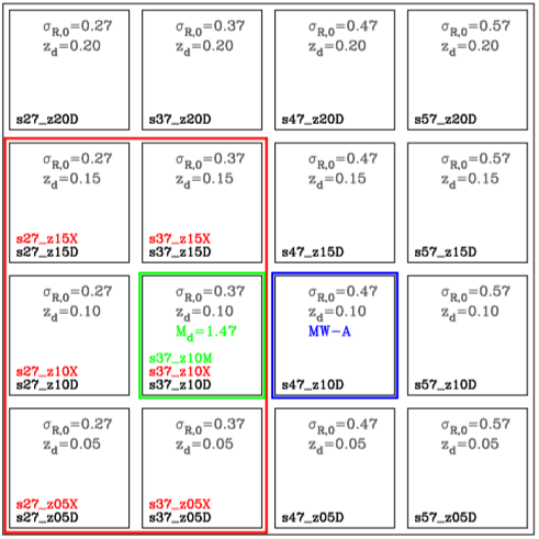
Fig. 1 This figure shows a grid of all our 26 simulations. The names of the models are given in the bottom left corner. The models have different disk central radial velocity dispersions σR,0 and disk scale height zd. These values are given in the upper right corner of each panel. Other parameters for the models are given in Table 1. The 16 black boxes correspond to models ran with 1.2 million particles. The blue box represents the MW-A model (Kuijken & Dubinski 1995). The red box shows models also ran with 8 million particles. The model in the green box was also ran with different numbers of particles and different disk masses (see Table 1). The color figure can be viewed online.
Table 2 Parameters of the modelsa
| model | N D | N B | N H | N G | m B /m D | m H /m D | M D /M G | M B /M G | M H /M G | M G |
| s27 z05D | 320000 | 80000 | 800000 | 1200000 | 1.92 | 2.32 | 0.14 | 0.07 | 0.80 | 6.24 |
| s27 z10D | 320000 | 80000 | 800000 | 1200000 | 1.95 | 2.26 | 0.14 | 0.07 | 0.79 | 6.25 |
| s27 z15D | 320000 | 80000 | 800000 | 1200000 | 2.00 | 2.25 | 0.14 | 0.07 | 0.79 | 6.24 |
| s27 z20D | 320000 | 80000 | 800000 | 1200000 | 2.05 | 2.27 | 0.14 | 0.07 | 0.79 | 6.25 |
| s37 z05D | 320000 | 80000 | 800000 | 1200000 | 1.92 | 2.32 | 0.14 | 0.07 | 0.80 | 6.24 |
| s37 z10D | 320000 | 80000 | 800000 | 1200000 | 1.95 | 2.26 | 0.14 | 0.07 | 0.79 | 6.25 |
| s37 z15D | 320000 | 80000 | 800000 | 1200000 | 2.00 | 2.25 | 0.14 | 0.07 | 0.79 | 6.24 |
| s37 z20D | 320000 | 80000 | 800000 | 1200000 | 2.05 | 2.27 | 0.14 | 0.07 | 0.79 | 6.25 |
| s47 z05D | 320000 | 80000 | 800000 | 1200000 | 1.92 | 2.32 | 0.14 | 0.07 | 0.80 | 6.24 |
| s47 z10D | 320000 | 80000 | 800000 | 1200000 | 1.95 | 2.26 | 0.14 | 0.07 | 0.79 | 6.25 |
| s47 z15D | 320000 | 80000 | 800000 | 1200000 | 2.00 | 2.25 | 0.14 | 0.07 | 0.79 | 6.24 |
| s47 z20D | 320000 | 80000 | 800000 | 1200000 | 2.05 | 2.27 | 0.14 | 0.07 | 0.79 | 6.25 |
| s57 z05D | 320000 | 80000 | 800000 | 1200000 | 1.92 | 2.32 | 0.14 | 0.07 | 0.80 | 6.24 |
| s57 z10D | 320000 | 80000 | 800000 | 1200000 | 1.95 | 2.26 | 0.14 | 0.07 | 0.79 | 6.25 |
| s57 z15D | 320000 | 80000 | 800000 | 1200000 | 2.00 | 2.25 | 0.14 | 0.07 | 0.79 | 6.24 |
| s57 z20D | 320000 | 80000 | 800000 | 1200000 | 2.05 | 2.27 | 0.14 | 0.07 | 0.79 | 6.25 |
| s27 z05X | 2133333 | 533333 | 5333334 | 8000000 | 1.92 | 2.32 | 0.14 | 0.07 | 0.80 | 6.37 |
| s27 z10X | 2133333 | 533333 | 5333334 | 8000000 | 1.95 | 2.26 | 0.14 | 0.07 | 0.79 | 6.35 |
| s27 z15X | 2133333 | 533333 | 5333334 | 8000000 | 2.00 | 2.25 | 0.14 | 0.07 | 0.79 | 6.35 |
| s37 z05X | 2133333 | 533333 | 5333334 | 8000000 | 1.92 | 2.32 | 0.14 | 0.07 | 0.80 | 6.37 |
| s37 z10X | 2133333 | 533333 | 5333334 | 8000000 | 1.95 | 2.26 | 0.14 | 0.07 | 0.79 | 6.35 |
| s37 z15X | 2133333 | 533333 | 5333334 | 8000000 | 2.00 | 2.25 | 0.14 | 0.07 | 0.79 | 6.35 |
| s37 z10M | 320000 | 80000 | 800000 | 1200000 | 1.09 | 0.72 | 0.33 | 0.09 | 0.59 | 4.44 |
| s37 z10MS | 320000 | 87449 | 577113 | 984562 | 1.00 | 1.00 | 0.33 | 0.09 | 0.59 | 4.44 |
| s37 z10MX | 2133333 | 533333 | 5333334 | 8000000 | 1.09 | 0.72 | 0.33 | 0.09 | 0.58 | 4.40 |
| s37 z10MXS | 2133333 | 586831 | 3775591 | 6495755 | 1.00 | 1.01 | 0.32 | 0.09 | 0.59 | 4.48 |
The first column is the name of the model which indicates some initial conditions (σR,0 and zd, see Figure 1). The number of particles of each component are given in Columns 2 to 4, and Column 5 shows the total number of particles for the system. Column 6 gives the mass ratio between bulge and disk particles, while Column 7 gives the mass ratio between halo and disk particles. Columns 8 to 10 give the total mass ratios of the components. Finally, Column 11 gives the total mass of the model MG.
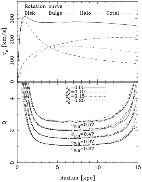
All our models generated similar rotation curves except those with the highest mass in the disk. As an example, Figure 2 shows the rotation curve resulting in model s27_z10D, and the initial Toomre stability parameter Q as a function of radius generated by the first 16 models listed in Table 2. The models with low values of Q will be called cold models, those with high values of Q, hot models. We will discuss the evolution of the Q parameter in § 3.3.
2.2. Temporal Evolution of the Models
The simulations performed in this work employed the N-body code gyrfalcON, based on the Dehnen (2000, 2002) force falcON solver (force algorithm with complexity) and the NEMO package (Teuben 1995). As do tree-codes, falcON begins by building a tree of cells at each time-step, then it determines the potential of the system using a multipole expansion for the cells and finally, it exploits the similarity of the force from a distant cell upon cells that are close to each other.
In all our simulations, we used a softening parameter ɛ= 0.05 and an opening angle θ=0.5. With these parameters, we ensured that the energy conservation was better than 104. The models were evolved from 0 to 5 Gigayears. Figure 3 shows six snapshots for models s27_z10D (top row) and s37_z10M (bottom row). The s27_z10D model formed transient spiral structures that faded after some rotations, and the s37_z10M model formed a bar structure that persisted throughout the entire evolution.
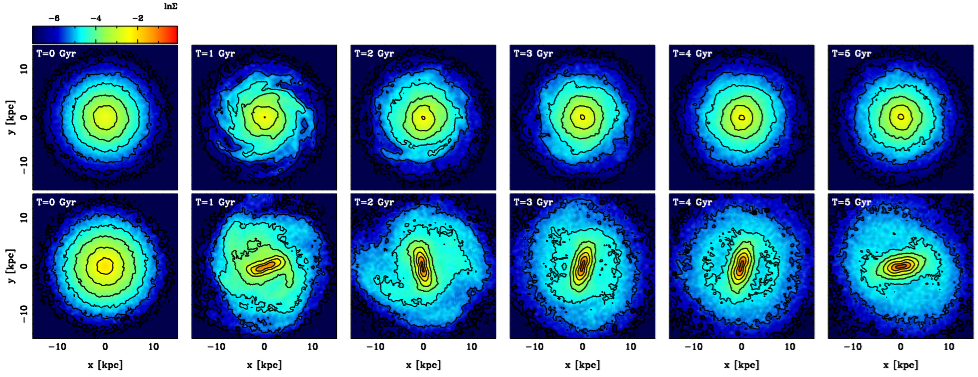
Fig. 3 Some snapshots of the models s27_z10D (top row) and s37_z10M (bottom row). The model with a light disk forms spiral structures which fade out after some rotations. The model with a heavier disk forms a bar, and this bar is maintained throughout the entire evolution. The time in Gigayears is given in the bottom left corner.
2.3. Analysis of the Models
We studied the time evolution of the models using one and two dimensional Fourier transforms (FT1D and FT2D, respectively). A high amplitude in the FT1D allows us to identify the region of the disk where the perturbation is strong and the FT2D allows us to get the pitch angle of the spiral structures. Thus, performing FT1D and FT2D over each snapshot shows how these modes (the structures) and their pitch angles evolve during the simulation. Moreover, the phase of the FT1D coefficients gives information about the pattern speed of the structures (bar and spirals). We use the bar pattern speed to study the orbits of the particles in the bar reference frame.
In order to implement the FT1D, we divided the disk into 100 rings at each time t (snapshot). Then, the FT1D was performed for each ring (R=1 to 100) as follows:
where
The FT2D method was applied to the distribution of the disk particles as described in Puerari & Dottori (1992) and references therein. We applied the FT2D in an annulus with a minimum radius of 4.5 kpc and a maximum radius of 15 kpc. The FT2D method was implemented using a logarithmic spiral basis,
Here,
3. RESULTS AND DISCUSSION
3.1. Unbarred Models
In this section, we present the calculations of the Fourier transform methods (FT1D and FT2D); for the models with 1.2 and 8 million particles which did not form a bar.
3.1.1. FT1D for Unbarred Models
We summarize the results of FT1D amplitude for all unbarred models in Figure 4. The mean amplitude of a given mode m for each model was computed for all times and radii. In this figure, the upper left panel shows the cold models, while the bottom right panel shows the hot ones. We found that the cold models develop the strongest structures at mode m = 2, but there are also some strong structures at modes m = 3 and m = 4; in fact, models s27_z05D and s27_z05X have a predominant mode at m = 2, due to the later formation of an inner oval and spirals. We conclude that the cold models are able to develop multi-armed structures, i.e. spiral structures with different azimuthal frequency number (m = 2, m = 3, m = 4), while it is clear that the hot models are unable to develop strong spiral structures with any azimuthal frequency.
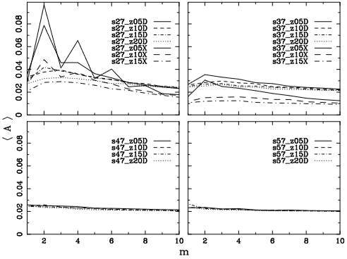
Fig. 4 Average amplitude < A > for modes m 1 to 10 for all unbarred models. The upper left panel shows the models with the lowest velocity dispersion (cold models) and the bottom right panel shows models with the highest velocity dispersion (hot models). While the coldest models generate the strongest structures at modes m = 2, m = 3 and m = 4, which is evidence of multiarmed structures, the hottest models do not generate structures.
In order to recognize where and when an m mode is amplified, we plot the Fourier coefficients AR(m) in gray-scale as a function of radius and time. Figure 5 is an example of these plots. The figure shows the amplitude of the FT1D for m = 2 between 2 and 3 Gigayears for the s27_z15D model. The regions with larger amplitudes (black stains) depict the growth of the structures. In this graph especially we can notice the evolution of an m = 2 structure appearing around a radial distance of 5 - 6 kpc. It is worth noting that at those distances the Toomre parameter Q is minimal. From there, the higher amplitudes move towards the inner and the outer parts of the disk.
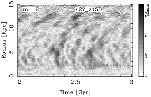
Fig. 5 Zoom of the FT1D for model s27_z15D for m = 2 as a function of radius and time. We can notice that the structures appear where the Toomre parameter Q is minimum (see Figure 2)
All our unbarred models follow this behavior. Furthermore, we notice that the perturbation begins to be amplified where the stability criterion is minimum, around 5 - 6 kpc (see Figure 2). It is known that models with low values of the Toomre parameter (1 < Q < 1.2), corresponding to cold models (Binney & Tremaine 1987), may develop non-axisymmetric structures via swing amplification, while models with high values of the Toomre parameter (Q > 2), corresponding to hot models, are unable to form structures in the linear regime. Indeed, our cold models (lower Q) are able to amplify strong non-axisymmetric structures (Figure 4).
Our next step is to measure the location and the pattern speed of the structures. Figure 6 shows spectrograms of the m = 2 perturbations as a function of radius over the entire evolution of these bisymmetric structures for four of our models. The darker areas correspond to the angular velocity of the strongest structures that are evolving in the disk. We note that these structures are located between the ILR and the OLR resonances, implying that there are different structures with different pattern speed at the same radius. Additionally, Figure 7 shows the pattern speeds of the s27_z15D model for different m modes illustrating that structures with different m’s can co-exist in the galactic disk. Like in Sellwood (2011), Sellwood & Carlberg (2014), Valencia-Enríquez & Puerari (2014) and Mata-Chávez et al. (2014), these figures suggest that a spiral structure is the result of the coupling of structures of an m mode and different pattern speeds, but also that they are coupling in different parts of the disk. The general morphology of our modeled galaxies is due then to the superposition of several different modes.
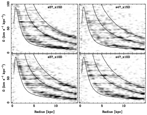
Fig. 6 Spectrograms giving the pattern speeds of the structures for some unbarred models with 1.2M particles for the m = 2 mode. The curves correspond to Ω + κ/2, Ω and Ω − κ/2. We note that the pattern speeds of the structures (dark regions) are well confined between the inner and the outer Lindblad resonances.
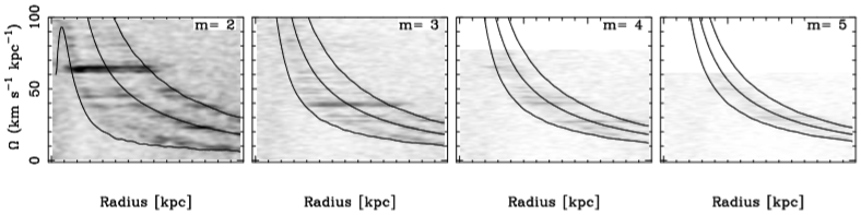
Fig. 7 Pattern speeds for the model s27_z15D for different m modes. The solid curves Ω and Ω ± κ/m correspond to the main resonances. Dark regions correspond to the pattern speed of the structures. It is clear that this model develops a multi-armed spiral structure. The pattern speeds of the structures for all m are well located between their main resonances
We also have evolved some models with a larger number of particles to investigate the growth of the spirals. We calculated models with 8 million particles (see Figure 1), i.e., we increased the number of particles by a factor of 6.6. Figure 8 shows the amplitude of the FT1D for different modes m as a function of time. The upper panel shows the amplitude for the s27_z10D model (with 1.2 million particles), and the bottom panel shows the amplitude for the same s27_z10X model (but with 8 million particles). These two panels are similar; this implies that the behavior of the model with more resolution is akin to the model with less resolution.

Fig. 8 These plots show the average amplitude |A| for modes m = 2, m = 3, and m = 4. We add 0.1 and 0.2 to the m = 3 and m = 4 for clarity. The mean was calculated over the radial range 3.75 to 12.75 kpc. The thickest line corresponds to mode m = 2, the intermediate thick line to mode m = 3, and the thinnest line to mode m = 4. The upper panel shows the amplitudes for the model with 1.2 million particles, and the bottom panel shows the amplitudes for the model with 8 million particles. These models generate multi-armed structures. Note that the model with low mass resolution generates structures earlier than the model with high mass resolution.
Therefore, all unbarred models (with both high and low resolution) have a similar behavior, as described before. However, the structures formed in the higher mass resolution runs appear somewhat later and are weaker than the structures formed in the lower mass resolution runs. It means that the heating of the disk for the high resolution models is weaker than the heating of the disk for low resolution models. The heating is due mainly to spiral activity and collisional relaxation. The collisional relaxation is a minor effect compared to the physically real collective heating caused by spirals. Hence, the high-resolution models have less heating because the spirals are weaker.
Fujii et al. (2011), Sellwood (2013) and Sellwood & Carlberg (2014) explored models with a different number of particles N in the disk. Fujii et al. (2011) found that the two-body relaxation has effects on the heating of the disk only when the number of particles is quite small, while Sellwood & Carlberg (2014) explained that the spiral activity causes the heating of the disk and the two-body relaxation is controlled by the softening in the force computation.
We must note that our models with high and low number of particles were calculated with the same softening. The high-resolution models heat somewhat later because the two-body relaxation is less important than in those with low resolution. The spiral activity in a high-resolution disk results in less heating than in a low-resolution disk because of the smaller amplitudes of the perturbations. We will strengthen this statement in § 3.3 where we discuss the evolution of the Q parameter for all models.
3.1.2. TF2D for Unbarred Models
We performed the FT2D on all our models, but for simplicity, we present in Figure 9 only the results for two models, with modes m = 2, m = 3, and m = 4. In this figure, each panel depicts the Fourier coefficient (the amplitude) |A(p, m)| on gray-scale as a function of time, and the frequency p. (see § 2.3). The highest amplitudes represent the spiral structures which are appearing in the disk, and the black stains show the evolution of these structures.

Fig. 9 The amplitudes of the FT2D for m = 2 for two of our unbarred models. Leading structures correspond to p < 0, and trailing ones correspond to p > 0. We can see that the amplitudes oscillated with time; these oscillations are due to the superposition of waves with different pattern speeds.
The oscillations present in the amplitudes of the spiral patterns are a signature of the superposition of structures - or modes - with different values of pitch angles and angular speeds. Such modes were already detected using the FT1D spectrograms (see e.g., Figures 6 and 7).
In the upper panel of Figure 10 we present a zoom of the FT2D amplitude for mode m = 2 between three and five Gigayears for the s27_z05D model, which is the coldest and thinnest model. In the bottom panel, we show a FT2D calculation where we simulated two different spirals with pitch angles of 14 and 12.5 degrees. One spiral rotates with an angular speed of 48 km/sec/kpc, while the other one rotates with Ω = 35 km/sec/kpc. The superposition of these two spirals gives a FT2D very similar to those we are measuring in our simulations. Then, we again emphasize that the Fourier analysis shows that the general morphology of our modeled galaxies is due to the superposition of several different modes.

Fig. 10 Upper panel: Zoom of FT2D at m = 2 amplitudes for the s27_z05D model. Spiral structures with different pattern speeds ‘beat’ as waves to give the appearence of periodicity in the amplitudes. Bottom panel: The FT2D calculated using two spirals with different pitch angles and angular speeds. The superposition of these two spirals gives a Fourier transform coefficient behavior very similar to that of our modelled galaxies.
All our models, including those with high and low mass resolution, follow this behavior, as was explained before. Moreover, the coldest/thinnest models generate strong spiral structures, while the hottest/thickest models do not generate structures. Sellwood & Carlberg (1984) argued that the spiral arms in N-body simulations generally fade over time because the spiral arms heat the disc kinematically and cause Q to rise. Our models also show this behavior when the Q parameter is increased. We study the effect of increasing Q in § 3.3.
3.2. Bar Models
In this section, we follow the analysis performed in § 3.1., but now on barred models. For these models, we also present an orbital analysis in order to show the growth of the bar.
3.2.1. TF1D for Barred Models
We ran models with a more massive disk (see Figure 1 and Table 2). These models clearly developed a bar feature because they had a quite small Q value at the beginning of their evolution because of the higher disk surface density.
We applied the FT1D in the same way as previously to analyze the growth of the bar and the spiral structures formed in the disk. The results of the FT1D are shown in Figure 11. Each panel of this figure shows, for each model, the mean amplitude < A > (equation 1) in logarithmic scale for m = 2 as a function of time and radius. These plots can be understood as growth curves of the structures that are being assembled. We observe that the evolution of the amplitude is similar among all barred models, the main difference being the bar’s growth rate. For example, the amplitude in the inner disk between 1 - 2 kpc for model s37_z10M (called bar fiducial model) reaches its maximum approximately at 0.9 Gyr, while for model s37_z10MX it reaches its maximum approximately at 1.4 Gyr. Also, while model s37_z10MS reaches its maximum approximately at 1 Gyr, model s37_z10MXS reaches its maximum much earlier, at 0.6 Gyr.
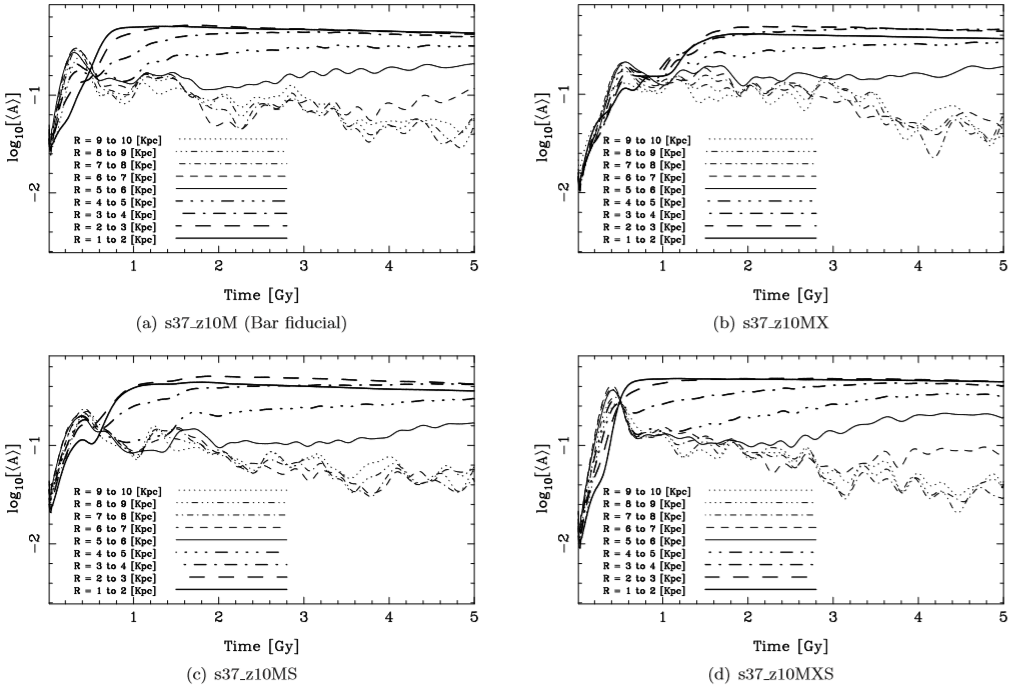
Fig. 11 The average of the FT1D amplitude for some radial ranges for the massive disk models for m = 2. Note that the amplitude for the inner radii grows and becomes more or less constant, representing the formation of the bar in the disk. The amplitude for the outer radii oscillates, representing the formation of transient spiral structures.
In order to calculate the instantaneous bar pattern speed as a function of time, we calculated the angle θ of the bar from the phase 𝛷 of FT1D for m = 2, taking the mean value of θ over a radial range from 0.15 to 2.25 kpc, thus obtaining a θ(t) curve. We then fitted a straight line for each 5 points on the θ(t) curve and took its slope for the middle point as the pattern speed Ωp(t). Figure 12 shows Ωp(t) for all barred models. It depicts the evolution of their instantaneous bar pattern speed showing that the bars appear with a high angular velocity, and that they slow down over time. Athanassoula (2014) showed that this decrease of the pattern speed could be explained as due to the angular momentum exchange within the galaxy or by the dynamical friction exerted by the halo on the bar. In a forthcoming article (Valencia-Enríquez et al., in preparation) we will present results focused on a large set of isolated/interacting barred galaxy simulations to gain insight on the processes which speed up or slow down the bar.

Fig. 12 The pattern speed of the bar as a function of time during the entire evolution for all barred models. The angular speed decreases in all models, from approximately 70−80 km/sec/kpc at the first Gigayear to 30−35 km/sec/kpc at end of our calculations, at 5 Gigayears.
In Figure 13 we present the m = 2 spectrograms of these simulations, now calculating them for three different time intervals (1 − 3, 2 − 4, 3 − 5 Gyr). This calculation allows us to compare the bar pattern speed and the spirals pattern speed. We can clearly observe the bar pattern speed in the inner part of the disk with high amplitude (dark horizontal line), and the pattern speed of the spirals in the outskirts of the disk with less amplitude.

Fig. 13 The spectrograms calculated for three-time intervals. We can see the bar slowdown over its evolution. It is also clear that the spirals rotate slower than the bar (see text).
The spectrograms of all barred models in Figure 13 show that the bar slows down more than the spiral. Furthermore, the bar rotates around twice as fast as the spiral structures. The spiral structure, as in the previous cases, results from the superposition of several m = 2 modes with different pattern speeds at different radial regions (see Minchev & Famaey (2010) for an extensive discussion on the spiral-bar resonance overlap). The difference between barred and unbarred models is that in barred models there are more m = 2 modes being amplified, probably due to the influence of the strong fast rotating central bar.
Also, we show the main resonance curves to identify whether the bar has an ILR. These results are shown in Figure 14. To plot these curves, we obtain Ω from the circular velocity of the model, and the main resonances from the equations Ω ± κ/2, where k is the epicycle frequency (

3.2.2. TF2D for Barred Models
For barred models with a heavier disk (green box in Figure 1), the FT2D was separately computed for both bar (0.1 < R < 4.5 kpc), and disk (4.5 < R < 15 kpc) regions. Figure 15 shows the Fourier coefficients of FT2D for the fiducial model; the results of the FT2D for the other barred models are very similar. The upper panels of this figure clearly show the presence of a bar structure; a very large amplitude appears for m = 2 and p = 0. The bottom panels show the spiral arms growing in the disk.
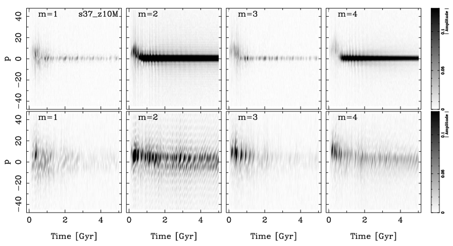
Fig. 15 The upper panels show the amplitude of the FT2D from m = 1 to m = 4 for the fiducial bar model. The FT2D was calculated over an inner radial region 0.1 < R < 4.5 kpc. The maximum amplitude found for the Fourier coefficient A(p = 0, m = 2) is a clear sign of the presence of a bar. The lower panels show the amplitude of the FT2D for the same modes m, but for the outer radial region 4.5 < R < 15 kpc. In the barred cases, the spiral structures are stronger than in the unbarred ones. For the outer radial region, larger azimuthal frequencies are triggered at the time of the bar formation.
Similarly to § 3.1.2, we zoom on the A(p, m = 2) coefficients in the interval between 3 and 4 Gigayears for the disk (4.5 < R < 15 kpc) region. These results are shown in Figure 16. We note that the spiral structures become stronger due to the presence of a bar (Buta et al. 2009) compared to those of the lighter disk simulation (see Figure 9), All in all, the spiral waves in this barred model have a similar behavior to the unbarred models. This is a clear evidence of the effect of the coupling of the spiral structures, now reinforced by the central bar.
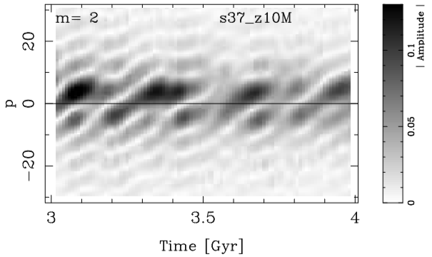
Fig. 16 Zoom of the FT2D amplitude at the m = 2 mode for the barred model calculated over the radial interval 4.5 < R < 15 kpc. Both leading (p < 0, with smaller amplitude) and trailing spiral structures (p > 0, with larger amplitude) appear at a given time due to the superposition of waves with different pitch angles and angular speeds. Note that the amplitude of these spirals is larger compared to that of the unbarred models (Figure 10).
3.2.3. Orbits for the Barred Models
We now focus our interest on an analysis of the disk stellar orbits in the bar reference frame. Chatzopoulos et al. (2011) proposed a complete analysis of the stellar orbits of test particles in gravitational potentials which is based on tracing patterns in sequences of characters, indicating sign changes of the Cartesian coordinates. We propose a very simple geometrical method in which we analyze three morphological types of orbits in the bar reference frame. For illustration, we show in Figure 17 the morphological evolution of six orbits for the fiducial barred model. We can clearly notice that a given particle is not confined to only one type of morphology; they change their morphologies during the entire evolution (Athanassoula 2012).
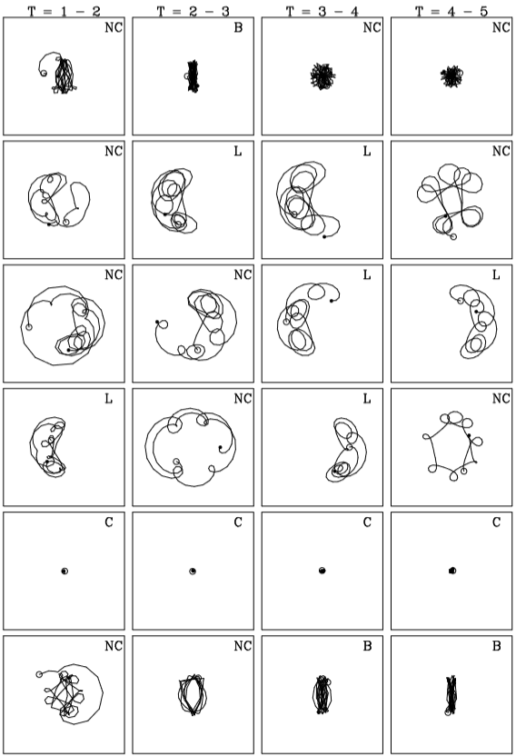
Fig. 17 Morphological evolution of six particles of the s37_z10M model. At each row, we plot the orbit of the same particle in four different time intervals. The orbit classification is given on the upper right corner. We observe that a particle is confined to an orbit type morphology, but it can change during the entire evolution.
In order to analyze the stellar orbits which evolved with the bar formation, we graphically classified the orbits of the disk particles in three primary morphological types as follows: orbits concentrated in the galactic center (compacts, C), orbits that run along the bar (bar, B), and orbits around the Lagrangian points L4 and L5 (loop orbits, L). We developed a code to identify these types of orbits taking our bar reference frame in a vertical position. We used the following criteria. To classify orbits as barred type we took |ymax| > 1.9|xmax| where |ymax| is the maximum value of a given particle in the vertical direction (along the bar) and |xmax| is the maximum position value of the same particle in the horizontal direction (perpendicular to the bar). The criterion to classify orbits as compact type was rmax ≤ 0.5 kpc, where r is the maximum radius of a given particle. Finally, the criterion to classify orbits as loop type was that the particle orbit remains confined to one side of the bar. Particles not following any of our three criteria were called unclassified (NC). These criteria were used for all disk particles at intervals of 1 Gyr.
Furthermore, we note that the bar appears around 1.5 Gigayears for the s37 z10MX model, and around 1 Gigayear for other models. Hence we made the orbital analysis from T = 1 to T = 5 Gigayear for all barred models. These results are shown in Figure 18. This figure shows the statistical classification of the three types of orbits weighted by the percentage of disk mass. The general behavior is similar for the all barred models. For example, as the bar forms, the number of compact orbits increases, and that of the loop orbits increases more. The number of bar orbits remains approximately constant after the second Gigayear.
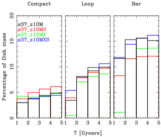
Fig. 18 Morphological classification for all disk particles orbits at four time intervals. The left panel shows the compact type orbits, the middle panel the loop type orbits, and the right panel the bar type orbits. At the end of our calculations (5 Gigayears) these three types of orbits encompassed approximately one-third of the disk mass (see text).
These models have the same initial conditions; the only difference is the number of particles, which defines their mass. This difference causes slight differences on how the noise affects the evolution of the models (Sellwood 2003). For example, we find that model s37_z10MS has more compact orbits than the other models, the number of loop orbits is almost equal to that of the fiducial models, and the number of bar orbits is approximately 4% fewer than that of the fiducial model. The largest model (s37_z10MX) keeps its compact orbits around 4% along its entire evolution. This model has 1.5% fewer loop orbits and 3% fewer bar orbits than the fiducial model after the second Gigayear. Finally, we can see that another large model, s37_z10MXS, closely resembles the fiducial model, with differences in the number of all type of orbits around 1%.
In general, the compact type orbits increase in number to encompass up to 5% of the disk mass, the loop type orbits increase in number to around 10% of the disk mass, and the bar type orbits increase in number to encompass around 15%, 13%, 12% and 16%. for the fiducial, s37_z10MX, s37_z10MS, and s37_z10MXS models, respectively. Finally, the three geometrically classified types of orbits, the ones trapped in the Lagrangian points L3, L4, and L5, encompass approximately one-third of the disk total mass for these bar models.
3.3. Toomre Stability Parameter Q
We have already discussed that the thickness of the disk zd affects the formation of non-axisymmetric structures. For example, Figure 4 shows that the models with a very thin disk (e.g. s27_z05D or s27_z05X) form stronger structures than do models with thicker disks, demonstrating that the local instabilities of the disk also depend on its thickness.
It is known that the stability of the disk is measured by the Toomre parameter Q in the standard first order perturbation scheme, where the disk is considered to be very thin and self-gravitating (Binney & Tremaine 1987; Bertin & Lin 1996). However, the thickness of the disk is also related to its stability (Q), and it is convenient to study Q for different values of the vertical scale height zd.
The measure of Q as a function of radius at three different times (0, 2.5, and 5 Gigayears) for unbarred models is shown in Figure 19, evidencing that the models with low/high velocity dispersion have low/high values of Q. Additionality, we note that the hotter models, in the upper panels, keep Q approximately constant throughout at time, while the initially colder models, in the bottom panels, show an increasing Q. Furthermore, this depends strongly on the initial disk thickness zd. For example, the increase of Q for model s27 z05D (or s27 z05X) is more conspicuous than that for model s27 z20D, which has a thicker disk. Hence, the stability of the disk should depend on the velocity dispersion in the z component (σz), the vertical scale height zd, and the mass of the disk. These results have also been discussed in Klypin et al. (2009).
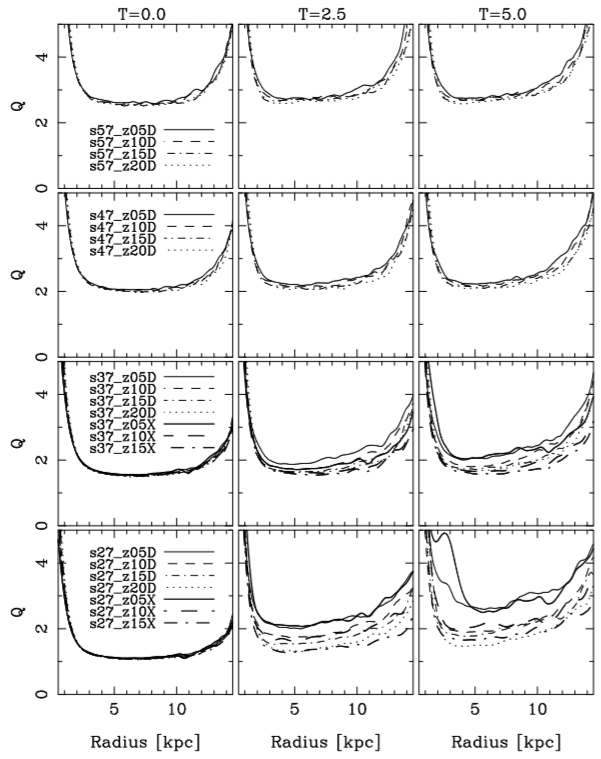
Fig. 19 The evolution of the Q parameter as a function of radius for all unbarred models. The Q parameter is shown at T=0, 2.5, and 5 Gigayears (see text).
We also measured the evolution of Q for barred models; these results are shown in Figure 20. We can see in this figure that Q is small at the beginning of the simulation, but that it increases quickly due to the bar and spiral formation. However, as the bar reaches its saturation and evolves far from the linear regime, the increase of Q does not affect the bar evolution nor the maintenance of the spiral structures.

Fig. 20 Evolution of the Q parameter as a function of radius for the barred models. The Q parameter for all barred models has small values at the beginning of the simulation, but it increases considerably due to the bar and spirals formation.
Additionally, we remark that the models with small and large number of particles and the same initial conditions heat the disk in a similar way (see Figures 19, and 20). Sellwood & Carlberg (2014) explained that this behavior is due more to the spiral activity than to two-body relaxation (Fujii et al. (2011)). It also depends on the softening parameter: if this is quite small, then the two body-relaxation could be important in the evolution of the model (Sellwood 2013), and the disk could quickly heat. See also (Romeo 1998) for an extensive study on the softening choice.
4. SUMMARY AND CONCLUSIONS
We performed a series of 3D fully self-consistent N-body simulations with 1.2 and 8 million particles. The initial conditions were chosen to follow the Kuijken-Dubinski models. We ran a grid of models with different disk radial velocity dispersion σR, disk scale height zd, number of particles N, and disk mass MD. We analyzed the growth of spiral structures by using one and two dimensional Fourier transforms (FT1D and FT2D). The FT’s give the amplitude, the number of arms, and the pitch angle of a particular spiral structure.
The FT1D proved to be a powerful tool to understand the growth of the spiral structures. The results of the FT1D show that the spiral structures emerge in the intermediate portion of the disk, where initially the Q parameter has its minimal value, and that these structures grow towards the outer parts of the disk with more intensity than inwards, due to the steep increase of Q towards smaller radii.
The plots of the FT2D amplitude as a function of time and pitch angle showed that the general morphology of our modeled galaxies is due to the superposition of structures with different values of p, m, and angular velocity.
We measured the angular velocity of all amplified patterns, and the results showed that these patterns are very well confined between the main resonances given by the Ω ± κ/m curves. Moreover, we found that different structures with either different or the same mode m and frequency p, and different pattern speeds can evolve in the same region of the disk at the same time. It is important to note that very often two or three different spiral structures can coexist in the same region of the disk.
Masset & Tagger (1997) showed a signature of non-linear coupling between the bar and spiral waves, or between spiral waves from modes m = 0 to m = 4. Similarly Sellwood (2011) showed that the bisymmetric spirals were not a single long-lived pattern, but rather the superposition of three or more waves which can grow and decay with time. We have shown that not only the spirals can overlap with different modes m, but also with different frequencies p. Thus, the general morphology of our modeled galaxies is due to the superposition of structures with different values for p, and m, i.e., different pitch angles and number of arms.
We remark again that the mass ratios MD/MG, MB/MG, MH/MG, and the initial conditions of models with small and large number of particles are equal, but the mass of the particles is different. Therefore, the evolution of these models is affected by noise (Sellwood 2003, Weinberg & Katz 2007a,b). For example, the bar in the model s37_z10M is formed earlier than in models s37_z10MX, probably due to our use of the same softening for all models. The noise increases more in models with fewer particles than in those with more particles. It is clear that by adding particles to the models the noise is reduced, and then the apparition of a bar or spirals is delayed (Sellwood 2003). However, all models have a similar behavior during all times, which means that the general behavior of the models is more affected by the spiral and/or bar activity than by the noise (Sellwood 2003).
Finally, we made an orbital analysis in the bar reference frame for those models where a bar formed. We proposed a very simple geometrical classification for three types of orbits: compacts, along the bar, and trapped near the Lagrangian points L 4 and L 5. Our main outcome was that after the bar formation, the number of compact orbits increases to reach around 5% of the disk mass; the loop like orbits increase to around 10% of the disk mass for all models; and the number of bar like orbits increases to attain around of 15%, 13%, 12% and 16% for fiducial, s37_z10MX, s37_z10MS, and s37_z10MXS models, respectively. Thus, we found that these three geometrically classified types of orbits, which are the ones trapped near the Lagrangian points L 3 , L 4 , and L 5 , encompass approximately one-third of the disk total mass for the barred models. Furthermore, a particle can change its orbit morphology during its evolution.
The authors gratefully acknowledge the very constructive comments offered by the referee, Jerry Sellwood, which improved the presentation of this paper. The authors also acknowledge support from the Mexican foundation CONACYT for research grants.

