


 nueva página del texto (beta)
 Inglés (pdf)
 Artículo en XML
 Referencias del artículo
 Enviar artículo por email
 Citado por SciELO
  Similares en
SciELO
Similares en
SciELO 
 Permalink
1. INTRODUCTION
The conventional methods of treating astronomical perturbations do not yield manageable series solutions for the motions of highly eccentric orbits (e.g. most comets and some asteroids) because they lie partly inside and partly outside the orbits of the disturbing bodies. Consequently, in applications of the conventional methods of expansion the disturbing force becomes a highly oscillating function, and results in divergent or at least very slowly convergent series expansions.
In an effort to overcome this situation, Hansen [1856] devised a method of computing the absolute perturbation of a periodic comet with large eccentricity based on the so called partial anomalies. This method involved division of the elliptic orbit of the perturbed body into segments. In each of the segments the classical variables (the true, eccentric or mean anomalies), were substituted by new ones: partial anomalies. The series representing the disturbing function was strongly convergent within the segment but invalid outside of it.
The first person to make full use of Hansen’s original method of partial anomalies was Nacozy (1969), who completed Hansen’s numerical example and compared the results with a numerical integration extending through 50 years. In his work, Nacozy utilized the pure harmonic analysis technique. In addition, the method was applied to the calculation of the general perturbations caused by Saturn on comet P/Tuttle (Skripnichenko 1972). All his analytical calculations were carried out by manipulating of Fourier series with numerical coefficients. In 1982, Sharaf proposed a regularization approach based on the idea of the orbit segmentation.
Originally, Hansen introduced two partial anomalies, the inferior anomaly denoted by k and the superior anomaly denoted by k 1. By means of these anomalies, the ellipse could be divided into two segments (as will be shown latter). Now one may ask: is it possible to divide the elliptic orbit into an arbitrary number of segments? The answer is yes, and can it be achieved firstly by a full understanding of the idea of the division of the elliptic orbit into two segments. The present paper is devoted towards this goal.
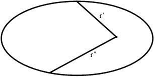
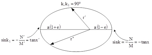
The idea of the segmentation may be stated as follows. As shown in Figure 1, let r ' be the radius to a point on the orbit between periapsis and apoapsis on one side of the major axis, where 0o ≤ E ≤ 180o, and let r '' be the radius to a point on the other side of the major axis, where 180o ≤ E ≤ 360o.
For the segment of the orbit containing the periapsis, we may consider the departure of r from r min = a(1−e).
This departure should satisfy the following conditions.
To be a periodic function of one independent variable.
To be positive ∀r between r’ and r’’.
To attain its maximum values at r and r , and its minimum value at a(1 − e). This departure therefore can be written as
where
The variable k is called the inferior partial anomaly.
For the segment of the orbit containing the apoapsis, we may consider the departure of 1/r from r min = 1/a(1 + e). This departure should satisfy the following conditions.
To be a periodic function of one independent variable.
To be positive ∀r between r ' and r ''.
To attain its maximum values at 1/r’ and 1/r’’ , and its minimum value at 1/a(1 + e). This departure therefore can be written as,
where
The variable k 1 is called the superior partial anomaly.
By means of these departures, many findings are established for both k and k 1, namely: (i) A transformation relating the eccentric anomaly to k and a transformation relating the true anomaly to k 1. (ii) Expressions for defining each of k and k 1 in terms of the orbital elements. (iii) The interpretation and the intervals of definition of two moduli (X, S) related to k and k 1. (iv)The extreme values of the radius vector r and the elliptic equations in terms of k and k 1. (v) That for two radii vectors, r ' and r '', the modulus X appearing in definition of the k and k 1 is a measure of the asymmetry of r ' (or r '') from r '' (or r '), while the modulus S 12 is a measure of the asymmetry of r ' and r '' from the minimum value of r. (vi) A description of the segments represented by k and k 1. (vii) The relative position of the radius vector at k = 0o and k 1 = 180o.
In what follows, we shall consider that the above equations are given and derive various conclusions associated with the segmentation, as well as provide additional interpretations to the parameters M, N, M ' and N ' appearing in these equations.
2. THE INFERIOR PARTIAL ANOMALY k
2.1. The equation defining k
This equation is,
where M + N and M − N are defined in equations (2), r ' and r '' are any two radii vectors of the ellipse. The expression relating the radius vector and the eccentric anomaly for elliptic motion is:
Upon comparing equations (5) and (6) one obtains:
as the transformation relating the eccentric anomaly to the inferior partial anomaly k. Also, by equation(6) we can write equations (2) as:
from which we obtain:
where E ' and E '' are the eccentric anomalies corresponding to r ' and r '' respectively. Further, setting
equations (5) and (7) could be written in terms of S 12 and X as:
Any one of the equations(5), (7), (13) or (14) could be used for the definition of the inferior partial anomaly k.
2.2. The equations defining S 12 and X in terms of r ' , r '' and in terms of E ' , E ''
From equations (11) and (12) we have:
Using equations (2) we can write equations (15) and (16) in terms of r ' and r '' as:
Using equations (9) and (10) we can write equations (15) and (16) in terms of E ' and E '' as:
Equations (17) and (18) are the required equations defining S 12 and X in terms of r ' and r '', while equations (19) and (20) are the corresponding equations in terms of E ' and E ''.
2.3. The intervals of definition for S 12 and X
Since for any radius vector r of the ellipse we have:
Consequently, for the two radii vectors r ' and r '' we have:
Equation (17) could be written as:
Then, by equations (24) and (25) this inequality becomes:
In addition, we can write equation (18) as:
and then
Using equations (22) and (23), the inequality (29) becomes:
and then we have:
Inequalities (27) and (31) are what we need to obtain.
2.4. The extreme values of the radius vector r and the elliptic equations in terms of k
Equation (13) could be written as:
Consequently,
The necessary condition for the extreme values of r is dr/dk = 0,
Therefore, the extreme values of r when expressed in terms of k occur at
Differentiating equation (33) with respect to k, we obtain:
Let us test the values of k given in equations (35) for the extreme values of r.
At k = 90o:
For this value of k, equation (36) becomes:
Since −π/4 ≤ X ≤ π/4, it follows that:
Consequently,
That is to say, at k = 90o ∀ − π/4 ≤ X ≤ π/4, r is maximum. Let this maximum be r 1. By equation (32) for k = 90o, we get for r 1 the value:
From equations (11) and (12) we obtain:
Using equations (9) and (10) in this equation yields:
Or
Using equations (43) and (17) in equation (40) it gives:
This equation could be obtained from equation (5) for k = 90o, by comparing the resulting equation with equations (2).
At k = 270o:
For this value of k, equation (36) becomes:
Again, since −π/4 ≤ X ≤ π/4, it follows that:
Consequently
That is to say, at k = 270o ∀− π/4 ≤ X ≤ π/4, r is maximum. Let this maximum be r 2. By equation (32) for k = 270o we get:
Using equations (43) and (17) in equation (48) yields:
This equation could be obtained from equation (5) for k = 270o, by comparing the resulting equation with equations (2).
At sink = −tanX = −N/M:
Equation (5) with sink = −N/M or equation (32) with sink = −tanX will give:
Therefore, at sink = −tanX r is minimum.
From the above analysis we have the following results.
Result 1:
The periodic representation of the radius vector r in terms of the inferior partial anomaly k [equation (5) or equation (13)] has two maxima, r '' and r ', when k = 270o and k = 90o respectively, and has a minimum a(1−e) when sink = −N/M or sink = −tanX.
Now we are in a position to obtain the elliptic equations in terms of k, and this is done as follows. We have already obtained the expression of r in terms of k as given in equation (32).
Since
And
we can write
where
Also, since
using the expression of sinE/2 in terms of k we obtain:
that is,
By equation (14) we have:
or
where A is given by equation (54).
Since
then
where n c is the mean motion. Equations (51) to (61) in addition to equation (32) are the required elliptic equations in terms of k.
2.5. Some remarks concerning the inferior partial anomaly k
It is evidently shown by the above analysis that certain points need discussion. In the following, some important remarks are given.
2.5.1. Interpretation of X and S 12
From equation (32) we have;
and
By these equations, and equations (18), (31) we have,
By these equations, and the equations defining S 12, the interpretation of X and S 12 may be as follows.
Result 2:
The modulus X appearing in the definition of the inferior partial anomaly k is a measure of the asymmetry of r '(or r '') from r ''(or r '), while the modulus S 12 is a measure of the asymmetry of r ' and r '' from the minimum value of r, which is a(1 − e).
2.5.2. Description of the segment represented by k
Equations (51) to (61), in addition to equation (32), show the following
At r = r '' ,k = 270o. As r decreases, k increases.
After passing the periapsis, r increases as does k, until at r = r ' we have k = 90o.
If we allow k to increase beyond 90o we retrace the same segment of the ellipse in reverse order.
Thus, we can describe the segment of the ellipse represented by the inferior partial anomaly k as follows.
Result 3:
The inferior partial anomaly k represents the segment of the ellipse from the periapsis to r = r ' on one side of the major axis, where 0o ≤ E ≤ 180o, and from the periapsis to r = r '' on the other side of the major axis, where 180o ≤ E ≤ 360o.
As k is varied from 0 to 360o, equations (5) or (13) and equations (7) or (14) give the coordinates of the ellipse, r and E, only in the segment formed by r ' and r '' as indicated in Figure 2 (in which r '' > r ').

2.5.3. Relative position of the radius vector at k = 0
Let the value of r at k = 0 be r 0; then, by equation (32) we have
From equations (62), and (65) we have;
and
Now we have to consider the following cases:
1. If r ' > r ''.
According to the first relation in (64), we have cosX < 2sin X, sinX > 0 and cosX > 0. Hence, by these conditions and equations (66) and (67) we have for this case;
2. If r ' < r ''.
According to the second relation in (64), we have cosX > 0 and sinX < 0. Hence, by these conditions and equations (66) and (67) we have for this case;
3. If r ' = r '' ≠ a(1 − e).
According to the third relation in (64) and equation (65) we have for this case;
From equations (68), (69) and (70), we may conclude the following result.
Result 4:
For r ' < r '' or r ' > r '', the radius vector r 0 corresponding to k = 0 lies on the same side of the major axis as the max{r ' ,r ''}, while for r ' = r '' ≠ a(1 − e), r 0 occurs at the periapsis. Figure 3 illustrates this result.
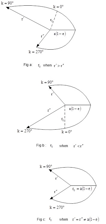
Fig. 3 Relative position of the radius vector r 0 for the three cases: r ' < r '' ,r ' > r '' and r ' = r '' ≠ a(1 − e).
This section completes the analysis of the inferior partial anomaly k. In the following section we shall consider the superior partial anomaly k 1.
3. THE SUPERIOR PARTIAL ANOMALY k 1
3.1. The equation defining k 1
This equation is:
where
The expression relating the radius vector to the true anomaly f for elliptic motion is:
Upon comparing (71) and (74) one obtains:
as the transformation relating the true anomaly to the superior partial anomaly k 1. From equation (74) we have:
From the analysis of § 2.5 we have f ' ≤ 180o and f '' ≥ 180o, then we must have:
and
Hence, by these equations, equations (72) and (73) could be written as:
hence
and
Let
By means of equations (82) and (83) we can write equations (71) and (75) in terms of
Any of the equations (71), (75), (84) or (85) may be used for the definition of the superior partial anomaly k 1.
3.2. Equations defining
From equations (82) and (83) we have:
Using equations (80), (81) we can write equations (86), (87) in terms of f ' and f '' as:
where f ' and f '' are the true anomalies at r ' and r '' respectively.
Using equations (72), (73) we can write equations (86), (87) in terms of r ' and r '' as:
3.3. The intervals of definition for
For any radius vector r of the ellipse we have:
consequently
and
Also for any radius vectors r ' and r '' we have:
Equation (90) could be written as:
where
Then by equation (95) the inequality (96) becomes:
In addition, we can write equation (91) as:
or
Where
and
By equation (94) this inequality becomes:
which gives
The inequalities (98) and (104) are what we need to obtain.
3.4. The extreme values of the radius vector r and the elliptic equations in terms of k 1
Equation (84) could be written as:
Differentiating equation (105) with respect to k 1 we obtain:
Since the necessary condition for the extreme values of r is dr/dk 1 = 0, then
Therefore, the extreme values of r when expressed in terms of k 1 occur at:
Differentiating equation (106) with respect to k 1 we obtain:
Now we shall test the values of k 1 given in equation (108) for the extreme values of r.
At k 1 = 90o:
For this value of k 1, dr/dk 1 = 0 and hence equation (109) gives:
Since −π/4 ≤ X ' ≤ π/4, it follows that:
By this condition, and the fact that
That is to say, at k
1 = 90o, ∀ − π/4 ≤ X
' ≤ π/4, r is minimum. Let this minimum be
By equation (105) for k 1 = 90o we get:
From equations (82) and (83) we get:
Using equations (80) and (81) in this equation gives:
or
Using equations (116) and (90) in equation (113) gives:
or
Then
This equation could be found from equation (71) with k 1 = 90o, by comparing the resulting equation with equation (73).
At k 1 = 270o:
Since for this value dr/dk 1 = 0, equation (109) gives:
Again, since −π/4 ≤ X ' ≤ π/4, it follows that:
From this condition, and from the fact that
That is to say, at k
1 = 270o ∀ − π/4 ≤ X
' ≤ π/4, r is minimum. Let this minimum be
By equation (105) for k 1 = 270o we obtain:
Using equations (116) and (90) in this equation, gives:
This equation could be found from equation (71) with k 1 = 270o, by comparing the resulting equation with equation (72).
At sin k1= −N′/M′=tanX′:
Equation (71) with sin k1−N ' /M ' or equation (105) with sink 1 = tanX ' will give:
Therefore, at sin k 1 = −N ' /M ' = tanX ', r is maximum. From the above analysis we can summarize
Result 5
The periodic representation of the radius vector r in terms of the superior partial anomaly k 1 [equation (71) or equation (105)] has two minima, r '' and r ', when k 1 = 270o and k 1 = 90o respectively, and has a maximum.
a(1 + e), when sink 1 = −N ' /M ' or (sink 1 = tanX ').
Now we are in a position to obtain the elliptic equations in terms of k 1. This is done as follows.
We have already obtained the expression of r in terms of k 1 as:
where
Since
then by using equation (85) we get cosf in terms of k 1 as:
Also, since:
where
then by equation (85) we get sinf in terms of k 1 as:
Since
then we can write:
Since
Hence, by using equation (135) in the left hand side of equation (134) we obtain:
Therefore, n c dt in terms of f is written as
Again, by equation (85) we have;
where C is given by (131).
Using equation (138) in equation (137) yields for n c dt in terms of k 1 the formula;
Equations (126), (129), (132) and (139) are the required elliptic equations in terms of k 1.
3.5. Some remarks concerning the superior partial anomaly k 1
Corresponding to § 3.4, the following remarks are given for the superior partial anomaly k 1.
3.5.1. The interpretation of X’ and
From equation (126) we have;
and
Using these equations, and equations (91), (104) we get;
By these equations, and the equations defining
Result 6:
The modulus X
' appearing in the definition of the superior partial anomaly k
1 is a measure of the asymmetry of r
'(or r
'' ) from r
''(or r
' ), while the modulus
3.5.2. Description of the segment represented by k 1
The elliptic equations in terms of k 1 show that:
At r = r ', we have k 1 = 90o. As r increases, so does k 1.
After passing the apoapsis, r decreases, k 1 increases until at r = r '' we have k 1 = 270o.
If k 1 increases beyond 270o, the same segment of the ellipse is retraced in the reverse order.
From these notes we can describe the segment of the ellipse represented by the superior partial anomaly k 1 as follows.
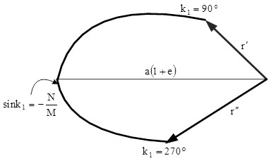
Result 7:
The superior partial anomaly k 1 represents the segment of the ellipse from the apoapsis to r = r ' on the side of the major axis where 0o ≤ E ≤ 180o, and from apoapsis to r = r '' on the other side of the major axis where 180o ≤ E ≤ 360o. As k 1 is varied from 0 to 360 , equations (71) or (105) and equations (75) or (85) give the′ ′′ coordinates of the ellipse , r and f, only in the segment formed by r and r’’ , as indicated in Figure 4 (in which r′′ > r′).
3.5.3. Relative position of the radius vector at k 1 = 180 0
Let the value of r at k
1
= 180o be
From equations (140), (141) and (143) we have
or
Now we shall consider the following cases.
1. If r ' > r ''.
According to the first relation in (142), we have cosX ' < 2sinX ', sinX ' > 0 and cosX ' > 0. Hence, by these conditions and equations (144) and (145) we have for this case
2. If r ' < r ''.
According to the second relation in (142), we have cosX ' > 0 and sinX ' < 0. Hence, by these conditions and equations (144) and (145) we have for this case
3. If r ' = r '' ≠ α(1 + e).
According to the third relation in (142) and equation (143)we have for this case
From equations (145), (146) and (147), we may state the following result.
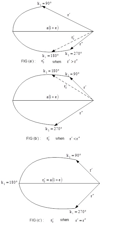
Result 8:
For r ' > r '' or r ' < r '', the radius vector r’0 corresponding to k 1 = 180o lies on the same side of the major axis as the min{r ' ,r ''}, while for r’=r’’≠α(1+e), r’0 occurs at the apoapsis. Figure 5 illustrates this result. This section completes the analysis of the superior partial anomaly k 1. This analysis leads to the following conclusions.
4. CONCLUSIONS
In the present paper, a novel analysis is given to show how Hansen’s inferior and superior partial anomalies k and k 1 can be used to divide the elliptic orbit into two segments (see Figure 6). The first segment includes the periapsis and is represented by the inferior partial anomaly k. The second segment includes the apoapsis and is represented by the superior partial anomaly k 1. The main findings of this manuscript can be summarized as follows.
The periodic representation of the radius vector r in terms of the inferior partial anomaly k has two maxima r’’ and r’ when k = 270o and k = 90o respectively, and a minimum a(1−e) when sink = −tanX.
The inferior partial anomaly k represents the segment of the ellipse from the periapsis to r = r′ on one side of the major axis where 0o ≤ E ≤ 180 and from the periapsis to r = r’’ on the other side of the major axis, where 180o ≤ E ≤ 360o.
For r ' < r '' or r′> r '' the radius vector r 0 corresponding to k = 0 lies on the same side of the major axis as the max{r’ ,r’’ }, while for r’ = r’’ ≠α(1 − e), r 0 occurs at the periapsis.
The periodic representation of the radius vector r in terms of the superior partial anomaly k 1 has two minima r’’ and r’ when k 1 = 270 and k 1 = 90o respectively, and has a maximum a(1+e) when sink = −tanX.
The superior partial anomaly k 1 represents the segment of the ellipse from the apoapsis to r = r′ on one side of the major axis where 0o ≤ E ≤ 180o and from the apoapsis to r = r’’ on the other side of the major axis, where 180o ≤ E ≤ 360o.
For r ' > r '' or r’ <′ r´’ the radius vector r’o corresponding to k 1 = 180o◦ lies on the same side of the major axis as the min{r’ ,r’’ }, while for r’=r’’≠α(1+e),
The authors are grateful to the referee for valuable comments that improved the original manuscript.

