


 nueva página del texto (beta)
 Inglés (pdf)
 Artículo en XML
 Referencias del artículo
 Enviar artículo por email
 Citado por SciELO
  Similares en
SciELO
Similares en
SciELO 
 Permalink
1. INTRODUCTION
Due to the presence of multiple turbulent layers in the atmosphere, the light coming from a distant astronomical object is refracted many times, and the images taken with a telescope are both blurred and shifted in the image plane (Kolmogorov 1941; Saha 2007). This degradation not only reduces the resolution of the acquired images well below the diffraction limit of the telescope, affecting the precision of astrometric measurements, but it can also degrade and complicate the photometry of dense stellar fields (Alard and Luption 1997). The blurring of astronomical images is also undesirable in spectroscopic observations, where a star has to be centered into a tiny slit of the spectrograph (Kitchin 1995). Moreover, the blurring makes ineffective the detection of light sources, as the object profiles overlap each other (Stetson 1987).
When using very fast acquisition (several tens or hundreds of frames per second) a point source (star) creates a dynamically evolving speckle pattern with a life time as short as several milliseconds in the visible (Voitsekhovich & Orlov 2014). Becauseof this, image enhancement techniques using either adaptive optics (Hardy 1998; Baranec et al. 2012) or software-based approaches, such as speckle interferometry (Tokovinin & Cantarutti 2008; Tokovinin et al. 2010), Lucky imaging (Law et al. 2006; Fried 1978), holographic imaging (Scho¨del et al. 2013) or image blind re-centering (Popowicz et al. 2015) require very short exposures, in which, unfortunately, only very few photons reach the detector. Moreover, counts from the sky background and the intrinsic noise of the sensor affect the quality of the measurements.
A special type of cameras, with electron multiplying CCDs (EMCCDs), was developed for acquiring images in such extremely low-light levels. They use the electron avalanche phenomenon to detect even single photons with high accuracy. This type of devices is frequently used in imaging techniques developed to overcome atmospheric degradation (Daigle el al. 2009). The recent availability of a new family of sCMOS sensors, with readout noise well below 1 e−, has taken scientific telescopes very close to reaching a perfect or ideal reception of photons.
The dynamic deformation of astronomical images caused by the atmosphere can be divided into two categories: tip-tilt (TT) effect and high-order distortions. While the latter can usually be compensated by adaptive optic tracking, frequently involving artificial laser guide stars, the former distortion is a simple shift of an entire speckle pattern that can be relatively easily corrected with a fast steering mirror (FSM). The latter type of correction requires splitting the light into two beams: (1) a beam following a path that leads through the FSM to a scientific CCD camera, taking relatively long exposures and (2) a beam following a path to a fast camera, that analyzes the temporal centroid position and applies compensations by adjusting the FSM tilt. The fast camera can be placed either after (close loop) or before (open loop) the FSM. It has been proven that TT is a dominant source of resolution degradation in small telescopes (<2 m) (Kevin et al. 2000) that may be made worse by instrumental factors, such as imperfections in telescope tracking. Importantly, the fast centroiding of a speckle pattern in very small telescopes (0.5 m in a good astronomical site), enables them to approach their diffraction limit (Watson et al. 2016).
Unfortunately, in telescopes with small apertures, the number of photons received in a single, short frame, is very limited, which can lead to errors in the position of the FSM, leading to an even larger degradation of stellar profiles. Thus, this study focuses on the possibility of TT correction using a matched filtering algorithm for the very low photon fluxes that are frequently received by small telescope systems. Our experiments aim at defining the limits for applying TT correction. We consider several factors that may influence the effectivity of TT correction, such as (1) the magnitude of the guide star, (2) the brightness of the sky background and (3) seeing conditions. Using a simulation of EMCCD imaging we compare how real acquisition changes the theoretical requirements imposed on TT guide star.
2. IDEAL PHOTON COUNTING
First, we simulated speckle patterns observed by an ideal photon-counting detector. To generate artificial speckle patterns, we employed the method of Random Wave Vectors (Kouznetsov et al. 1997; Voitsekhovich et al. 1999), which allows to accurately imitate a wide range of atmospheric effects, including TT. Since this study focuses mainly on small telescopes, we used a D/r 0 parameter ranging from 1 to 7 for an assumed small telescope (e.g. 0.3 m), this corresponds to a Fried parameter of r 0 = 4 to 50 cm, which covers the most frequent seeing conditions in both the visible and the infrared at good observing sites. A single image returned by the random wave vector simulation has 1024×1024 pixels, which means that each of the simulated images can contain an entire speckle pattern. In our data an image pixel corresponds to λ/4D, which ensures that the sampling frequency is two times higher than that required by the Nyquist limit. A series of 1000 images was generated for each value of D/r 0 . The upper row of Figure 1 shows examples of simulated speckle patterns; the lower row shows the long-exposure outcome for each corresponding series.

Fig. 1 Examples of speckle patterns generated using the Random Wave Vector algorithm. Above: examples of single frames, Below: average of 1000 images (long exposure outcome). From the left: D/r 0 = 1,3,5 and 7.
To find the most accurate centroid position of very noisy data, it is more appropriate to use the matched filtering approach instead of a simple centroid algorithm, as it is more effective when dealing with extremely low-light-level observations (Popowicz et al. 2015). To obtain the TT offset of each image, it is necessary to obtain an expected speckle profile (matched profile), and then convolve each image with it. The maximum in the resulting convolved image indicates the most probable position of the speckle centroid. In speckle patterns, for which very few photons are recorded, it is generally not possible to obtain an average speckle profile without ideal TT correction. Therefore, we assumed that a simple average of the whole series (i.e. without TT correction) (lower row of Figure 1) could be used as the matched profile for a given D/r 0 .
Initially, we studied how the overall TT error behaves for various D/r 0 using the simulated series. As a measure of image drift, we used the root mean square distance, ∆RMS, between the center of the image (expected centroid position) and the actual centroid. We observed a clear linear dependence, as can be seen in Figure 2. This effect is also clearly visible in individual speckles (Figure 3).
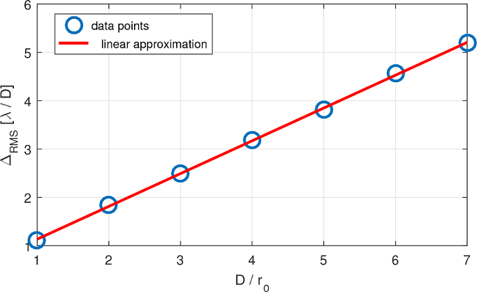
Fig. 2 RMS tip-tilt error of the speckle centroid as a function of the relative seeing conditions (D/r 0 ).
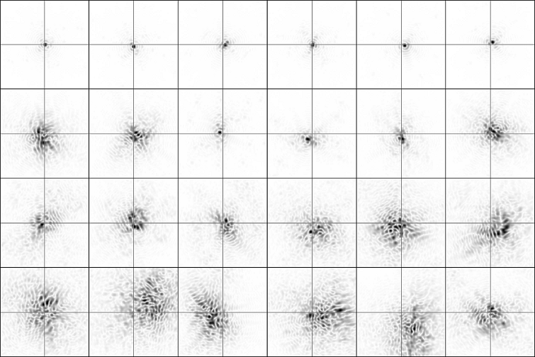
Fig. 3 Effect of tip-tilt correction on simulated speckle patterns. Each row corresponds to different seeing conditions: D/r 0 = 1, 3, 5 and 7 from top to bottom, respectively. The gray auxiliary lines indicate the expected centroid position, i.e. the center of the frame. The color figure can be viewed online.
One should remember that the speckle pattern becomes more complex as D/r 0 increases, and the correction is not as effective as for smaller values of D/r 0 . For comparison, Figure 4 shows the effects of an ideal TT correction for four values of D/r 0 . In addition, the plot on the right shows the maximum Strehl ratio1 that can be achieved with and without an ideal TT correction for various D/r 0 . It can be seen that for large D/r 0 there is virtually no benefit from the TT correction.
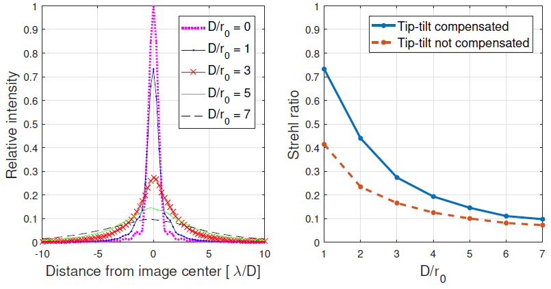
Fig. 4 Comparison of the results of tip-tilt correction for various D/r0 scenarios. Left: cross-section of stellar profile with ideal tip-tilt correction. Right: Strehl ratio achieved with (solid line) and without (dashed line) tip-tilt correction. The color figure can be viewed online.
To study the effect of a low number of recorded photons on the effectiveness of the TT correction, we used simulated speckle patterns as a reference of flux distribution. We assumed three different telescope diameters (0.3 m, 0.5 m and 1 m), a narrow V photometric filter (90 nm width), and a exposure time of 0.01 second, in which TT effects, even in the visible, remain virtually frozen. To calculate the expected number of photons in a speckle of a star between 11 and 17 magnitude, we downscaled the known flux of a zero magnitude star (1000 photons/cm2/s/A, in the visible) and multiplied it by the average attenuation of the atmosphere and of the entire telescope system (mirrors, filters, image sensor)2. The simulated, photon-limited speckle patterns that accounted for the Poisson distribution of counts were contaminated with random photons from the background in proportion to a given sky brightness: 19, 20, 21 and 22 mag/arcsec2, respectively. Example results of the simulation for a 1 m telescope are shown in Figure 5. The differences between sky background intensities become noticeable for stars fainter than approximately 14 mag. This agrees with the results of our analysis which are presented in another section of this paper.

Fig. 5 Examples of simulated speckles (negative, D/r 0 = 4) for a 1 m telescope and for a range of star magnitudes and background sky levels. Each image was normalized so that the black level corresponds to the maximum intensity in a speckle.
We then calculated the centroids for all low-lightlevel speckles and compared them with the ideal centroids to obtain the RMS error of the centroid estimation ∆RMS. Figure 6 shows examples of the results obtained for a 0.5 m telescope and D/r 0 = 1, 4 and 7. The marks indicate the measurements while the solid lines are cubic interpolations of data points. Since we are interested in the minimum brightness of a guide star that allows for any any improvement of image quality, a dashed horizontal line was added to the plots, to show the RMS centroid error of a system without TT correction. As expected, the RMS error increased significantly above the reference dashed line when the star intensity decreased, which implies that a TT correction becomes infeasible when not enough photons are received from a star and/or when the signal-to-background ratio is very low. As can be seen in Figure 6, for an assumed 0.5 m telescope, the guide star should always be brighter than 15 magnitude. The correction is obviously affected by sky brightens, and so it works best in darker sites.

Fig. 6 The RMS error of the speckle centroid (∆RMS) for a 0.5 m telescope. Left: results for D/r 0 = 1, 4 and 7. The horizontal dashed line in each plot indicates the RMS centroid error for observations without TT correction. The color figure can be viewed online.
To better study the effect of D/r 0 on the minimum required magnitude of the guide star, we determined the magnitude at which the curves in Figure 6 cross the reference dashed line. For this, we used the interpolations represented by solid lines in Figure 6 The results for the three telescope sizes, together with their linear approximations, are shown in Figure 7. It can be seen that the larger the D/r 0 ratio, the brighter the guide star has to be. Moreover, for very bright sky backgrounds, this dependence is steeper, meaning that the required intensity of the star is more sensitive to seeing conditions. Obviously, using a larger telescope allows for fainter guide stars.
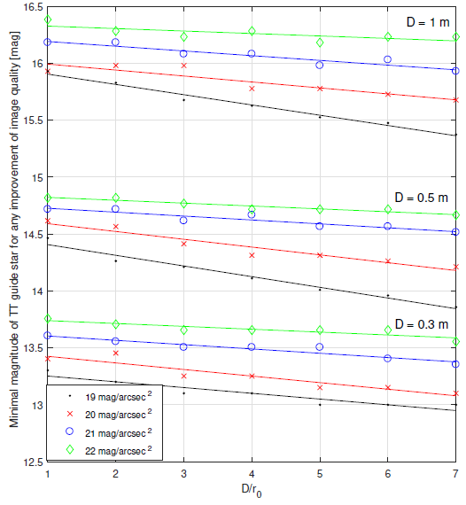
Fig. 7 Dependency of the minimum intensity of the TT guide star that allows for any improvement in image quality, under relative seeing conditions D/r 0 , different brightness values of sky background, and three telescope sizes: 0.3 m, 0.5 m and 1 m. Since the dependencies are clearly distinguishable, they are presented in one plot. The color figure can be viewed online.
The results of our evaluations can be also presented in the form of dependencies of the magnitude of a guide star as a function of telescope aperture for various seeing conditions expressed by the Fried paramter r 0. We summed up these results in four plots presented in Figure 8; each plot corresponds to a different intensity of the sky background. As can be observed, under poor background conditions (i.e. 19 mmag/arcsec2), the TT correction is much more dependent on seeing conditions r 0, compared to very dark sites. This was also noticeable in Figure 7.
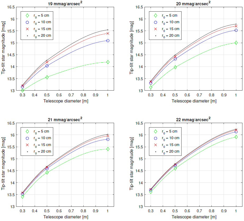
Fig. 8 Dependency of the required minimum intensity of the TT guide star and telescope size for various seeing conditions expressed by the Fried parameter r0, and for four intensities of sky background. The marks show the measurements; solid lines are cubic interpolations. The color figure can be viewed online.
3. EFFECT OF NOISE ON EMCCD IMAGING
The most popular type of cameras for fast imaging are electronic multiplying CCD (EMCCD) cameras. In this type of image sensor, the charge is multiplied along the horizontal register, so that the output of electrons is much larger than the readout noise. Thus, the effective readout noise (compared with the scale output) of EMCCDs can be as small as 0.01 e−. The drawback is that it is difficult to estimate the number of input electrons. If n photoelectrons are recorded in each EMCCD pixel, after the multiplication, the output number of electrons m follows the distribution (Popowicz et al. 2016):
where P(m) is the probability of receiving m output electrons; g stands for the charge gain parameter set by a user, which can be as high as 1000 in an Andor iXon888, state of the art, EMCCD camera. The higher the gain, the lower the effective readout noise, which becomes σ e /g, where σ e stands for the readout noise in CCD images (no multiplication used). Therefore, as long as there is no saturation of pixels, this parameter should be set to the maximum value allowed by the manufacturer.
To study how the image formation process of EMCCDs influences the effectivity of TT correction, we converted the photon counts obtained in the experiment described in the previous section, using the distribution from Equation 1. In addition, we contaminated each pixel with a readout noise σ e = 10 e− (Gaussian distribution), which is a typical value for the best current EMCCD cameras working in very fast imaging modes. Taking all the steps in the same way as it would be done for ideal photon-limited images, we obtained the dependency of the required magnitude of the TT guide stars, as shown in Figure 9. Figures 8 and 9 show a comparison between ideal and realistic results of the TT correction in very small telescopes. To better show the increase in the minimum intensity of the TT guide star (∆ TT star ) after including the realistic image formation process of the EMCCD camera, we compared the curves from Figures 8 and 9; the result is shown in Figure 10.

Fig. 9 Dependency of the required minimum intensity of the TT guide star and telescope size for a realistic EMCCD imaging process, under various seeing conditions represented by the Fried parameter r0, and for four intensities of sky background. The limits of the y and x axis were adopted from Figure 8. The marks show the measurements; the solid lines are cubic interpolations. The color figure can be viewed online
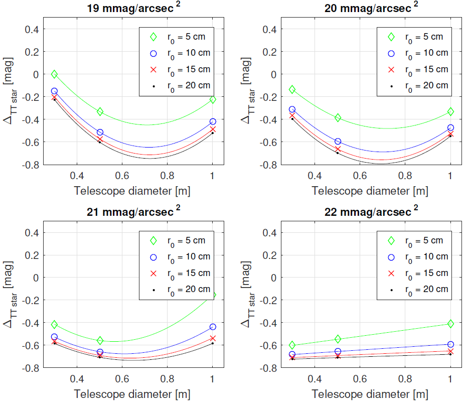
Fig. 10 Difference in the minimum intensity of the TT guide star between ideal and EMCCD imaging, (∆TT star). This figure shows the difference between the results presented in Figure 8 and the results presented in Figure 9. The negative values indicate the increase of the required intensity of the TT guide star. The marks show the measurements; the solid lines are cubic interpolations. The color figure can be viewed online
Figure 10 shows that the intensity of the TT guide star required to achieve any improvement in image quality has to be on average 0.5 mag brighter (0≈0.8 mag) than the result for an ideal imaging process. These differences are larger if the observations are performed under a very faint (22 mag/arcsec2) sky background. This can be explained by the high quality of the centroid estimation of the ideal detector when the background noise is low, which unfortunately decreases significantly when the readout noise appears. It seems that, for such low sky backgrounds, the sky coverage allowed by the TT correction can be improved by using less noisy photon detectors.
All plots in Figure 10 show that the difference ∆ TT star disappears when the aperture of the telescope increases. This is due to the large spatial spread of photons in a speckle pattern (larger D/r 0 ), which improves the quality of the centroid estimate by reducing its sensitivity to the multiplicative noise induced by the EM register. Furthermore, the decrease of ∆ TT star is also visible in the plots on the left side, i.e. for a 0.3 m telescope (except for the last plot, corresponding to 22 mag/arcsec2). We suppose that this effect is related to a high concentration of the stellar profile, which also allows to overcome the disadvantages of the multiplicative noise.
A kind of minimum is visible in the three plots of Figure 10. It indicates the size of telescope for which the realistic imaging results cause the largest increase of the required intensity for the TT guide star. This minimum moves toward smaller apertures for fainter sky backgrounds, and so it is not visible in the fourth plot. This indicates that smaller telescopes do not suffer so much from the realistic imaging processes as long as they work under high-intensity sky backgrounds and poor atmospheric conditions.
It is worth noting that, in addition to the increase in the minimum intensity of the TT guide star, the effect of seeing conditions on the TT guide star becomes less important. This is evidenced by the smaller spread of the curves in all plots of Figure 10. For a sky background of 22 mag/arcsec2, all the dependencies nearly overlap.
4. SKY COVERAGE
Finally, we present how the intensity of the guide star can be translated into the sky coverage allowed by the TT correction. For this, we used a rough estimation of the distrubution of stars of a given magnitude, such as that provided by Hardy (1998). To obtain more accurate models of sky coverage, if required, an interested reader is kindly referred to Robin et al. (2003). For this work we decided to use a simpler method, since our aim was only a brief inspection of possible sky coverage. Depending on the position of observed field, two estimates of the number of stars per square radian are given by the following formula (Hardy 1998):
Galactic equator:
Galactic pole:
Average:
where m V stands for star magnitude in the V photometric filter. To assess the sky coverage, Figure 11 shows the plots for a range of isoplanatic angles of TT. In contrast to the isoplanatic angle of high-order distortions, which are the same only within small angles (up to several arc seconds in the visible), TT effects are correlated over much wider fields; therefore we selected isoplanatic angles of 30′′, 60′′and 120′′for the calculations.

Fig. 11 Sky coverage as a function of the magnitude of the guide star. Left: dependencies for Galactic equator, Galactic pole and for an average stellar field. Red, green and blue colors in each figure correspond to the assumed isoplanatic angle of TT effects: 30′′, 60′′and 120′′, respectively. The color figure can be viewed online.
Based on the results of previous sections, it appears that the average sky coverage of small telescopes (≈ 0.3 − 1m) equipped with TT correction ranges between: ≈ 15 − 100% for 120′′ TT isoplanacity, and ≈ 5 − 25% for 60′′ TT isoplanacity, ≈ 2 − 10% for 30′′ TT isoplanaticy.
5. SUMMARY
Tip-tilt correction is the simplest method to improve the quality of astronomical images. It can be very effective for very small telescopes (≤ 1 m), which are usually used when relative seeing conditions, D/r 0 , are very good. TT correction allows small telescopes to almost reach their diffraction limit. Unfortunately, the small number of photons received by small telescopes creates significant difficulties in the estimation of the temporal centroid of a speckle pattern.
In this work we evaluated how various factors, namely, seeing conditions, sky background and telescope size, influence the minimum intensity of the TT guide star required to achieve any improvement of image resolution. Using the Random Wave Vector method, we simulated speckles for decreasing values of D/r 0 to imitate real photon detections in the image plane. The results of our simulations include a series of plots that predict the required magnitude of the TT guide star for various telescope sizes under various seeing/sky background conditions.
The outcomes of real detections performed by EMCCDs were simulated to assess the change in TT requirements compared with an ideal photon counting detector. We found that, on average, guide stars 0.5 magnitude brighter (≈ 0−0.8mag, depending on conditions and instruments) are needed to perform TT correction with a real photon detector. Interestingly, the smallest telescope included in our simulations (0.3 m), working under poor atmospheric conditions and with high sky background, showed virtually no differences in efficiency between an ideal and a realistic imager. This suggests the benefits that could be obtained by employing TT correction at poor observing sites.
The results of this work can also be used for predicting the maximaum sky coverage of very small telescopes equipped with a TT compensator. They can be used during the development stage of smallaperture instruments, like the one described in Watson et al. (2016), to estimate their detection capability at certain observing sites where the atmospheric conditions and the sky background are well characterized.

