


 nova página do texto(beta)
 Inglês (pdf)
 Artigo em XML
 Referências do artigo
 Enviar este artigo por email
 Citado por SciELO
  Similares em
SciELO
Similares em
SciELO 
 Permalink
1. Introduction
The Orion nebula is the brightest H II region in the night sky. It is considered the standard for studying the chemical composition of H II regions and the mechanisms that play a role in the evolution of these objects. Herbig-Haro (HH) objects have been studied extensively in molecular clouds, where they can be observed in the infrared. For H II regions the work has centered mostly on the physical conditions and morphology of these objects (e.g. Reipurth & Bally 2001; O’Dell & Henney 2008; Smith et al. 2010). Only a few photoionized HH objects have been identified and chemically characterized in HII regions, notably HH 529 (Blagrave et al. 2006) and HH 202 (Mesa-Delgado et al. 2009a) in the Orion Nebula.
HH 202 is the brightest Herbig-Haro object discovered yet. It was first identified by Cantó et al. (1980). Its characteristics allow us to resolve and study the gas flow with high spatial resolution. The parent star has not been identified. However, the shock is expanding to the NW and appears to be related to nearby HH objects HH 529, 203, 204, 528, 269, and 625. The kinematics of the object are well known; O’Dell & Henney (2008) report a radial velocity between −40 and −60 km/s, while Mesa-Delgado et al. (2009a) conclude that the bulk of emission comes from behind the flow. The object consists of several knots, of which the southern knot (referred to as HH202-S) is the brightest.
HH 202 has been studied previously by Mesa-Delgado et al. (2009a) with the UV ES echelle spectrograph of the Very Large Telescope, and Mesa-Delgado et al. (2009b) using integral field spectroscopy. The first work is particularly relevant as it presented an in-depth, high precision analysis of the physical conditions and the chemical composition of the shock. They observed an area of 1.5 × 2.5 arcsecond2 of the sky covering the brightest part of HH 202-S. Their high spectral resolution enabled them to separate the emission from the static gas and the shock. They showed that the heating is due mainly to photoionization by θ1 Ori C, effectively showing that HH 202 can be characterized as an H II region. They also determined its chemical composition including the presence of thermal inhomogeneities along the line of sight by means of the t2 parameter first proposed by Peimbert (1967). Finally they calculated the amount of dust destruction and oxygen (O) depletion.
Although echelle spectrographs provide high spectral resolution, the observed area of the sky is limited to a few arcseconds2. For this reason a longslit study -which, in the case of FORS 1, allows the study of a 410′′× 0.51′′region- of the same area of the sky, is excellent to complement and contrast previous results and allows the spatial exploration of parameters.
The chemical composition of an H II region is usually inferred from its emission spectrum. However, this only represents the gaseous abundance of elements. It is necessary to account for the fraction of a species depleted into dust in order to obtain the total abundance of an element; typically this is reported as a quantity that must be added to the gaseous abundance. Some interstellar shocks are capable of destroying interstellar dust grains if they are energetic enough (Mouri & Taniguchi 2000); this phenomenon has been reported in supernova events (Gall et al. 2014) and Herbig-Haro objects (Podio et al. 2009; Mesa-Delgado et al. 2009a).
The case of oxygen trapped in interstellar dust is particularly interesting as it is the third most abundant element in the interstellar medium. The shock velocity of HH 202 is capable of destroying dust grains; this makes it a good candidate to study the incorporation of oxygen and other elements from the dust phase into the gas phase. Esteban et al. (1998) and Mesa-Delgado et al. (2009a) have estimated the depletion correction for oxygen to be 0.08 dex and 0.12 ± 0.03 dex respectively.
In this work, we conduct an analysis of HH 202 using the long-slit Focal Reducer Low Dispersion Spectrograph 1 (FORS 1) of the Very Large Telescope. In § 2 we present our observations and the data processes we used. We perform a spatial analysis of the iron (Fe) and oxygen emissions in § 3, including the spatial variation in abundance across the Orion nebula. In § 4 we present our results combining multiple spectra and identifying the zones where the shock due to HH 202 is most prominent; electron density and temperature are calculated and ionic and total abundances are presented assuming constant temperature and thermal inhomogeneities. Finally we calculate the oxygen depletion inferred from dust destruction and present the conclusion of our analysis in §5 and §6.
2. Observations and data reduction
The observations were carried out during the night of September 11, 2002 with FORS 1 at the Very Large Telescope (VLT), in Cerro Paranal, Chile. Data were obtained from three different grism configurations: GRIS-600B+12, GRIS-600R+14 with filter GG435+31, and GRIS-300V+10 with filter GG375+30 (see Table 1).
Table 1 Journal of observations
| Grism | Filter | λ (Å) | Resolution (λ/∆λ) | Exposure time (s) |
| GRIS-600B+12 | … | 3450-5900 | 1300 | 3 × 60 |
| GRIS-600R+14 | GG435 | 5250-7450 | 1700 | 5 × 30 |
| GRIS-300V | GG375 | 3850-8800 | 700 | 3 × 20 |
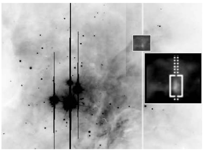
An image of the Orion Nebula from our observations is shown in Figure 1. The slit was oriented North-South, and the atmospheric dispersion corrector was used to keep the same observed region within the slit, regardless of the airmass value. The slit length was 410′′and the width was set to 0.51′′. This setting was chosen to have enough resolution to deblend the [O II] λ3726 and λ3729 emission lines, as well as to measure O II λ4642 and λ4650 with a significant signal to noise ratio with GRIS-600B+12.
The final spectrum was reduced using IRAF4 following the standard procedure of bias substraction, aperture extraction, flat fielding, wavelength calibration and flux calibration. The standard stars used for this purpose were LTT 2415, LTT 7389, LTT 7987, and EG 21 (Hamuy et al. 1992, 1994). The error in flux calibration was estimated to be 1%.
To analyze the spatial variations of the physical properties and of the chemical abundances 54 extraction windows were defined. Windows North and South of HH202-S spanned 50 pixels (10”.) each, whereas those covering the object were 3 pixels (0.6’’.) long each. This treatment of the data allowed us to establish the composition of the Herbig-Haro object and to compare it directly with the surrounding gas of the Orion nebula. The apex of HH202-S -that is, the region where the shock is strongest- has coordinates (J2000.0): α=05h35m11s. 6,δ=−5°22’56’’.The apex was determined from the peak of emission of [Fe II] λ7155; [Fe III] λ4658; O II λλ4640 and 4652; and Hα.
3. Spatial analysis
We performed an analysis of the flux of a set of emission lines in all 54 windows: the Balmer series up to H9; [Fe II] λ 7155; [Fe III] λ 4658; and O II λλ4640 and 4652. The flux of the emission lines was determined by integrating between two points over the local continuum estimated by eye. This was done using the SPLOT routine of IRAF. A Gaussian profile was fitted to the lines that were blended together. The results for Hα are presented in Figure 2 showing a peak that coincides perfectly with the brightest section of the slit covering the object (Figure 1). This peak also coincides with the peak of the iron emission lines presented in Figure 3, indicating the center of the shock.
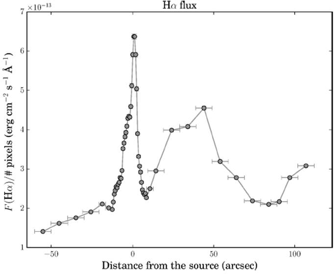
Fig. 2 Hα flux across the Orion Nebula. The zero mark was determined from the peak of [FeIII] emission with approximate coordinates α = 05h35m11s.6 and δ = −5°, 22’, 56’’.2 (2000). North is to the left of the zero mark and South is to the right.
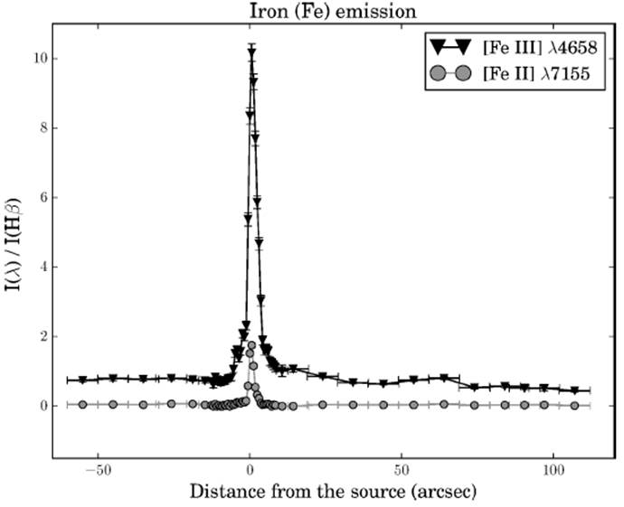
Fig. 3 Dereddened emission line intensities for [Fe II] λ7155 and [Fe III] λ4658 across the Orion Nebula.
We tested the extinction laws of Seaton (1979), Cardelli et al. (1989), and Costero & Peimbert (1970). The logarithmic extinction correction for Hβ, C(Hβ), and the underlying absorption were fitted simultaneously to the theoretical ratios. The theoretical intensity ratios for the Balmer emission lines were calculated using INTRAT by Storey & Hummer (1995) considering a constant electron temperature Te = 9000 K, and an electronic density ne = 5000 cm−3; there was no need to modify these values since the hydrogen lines are nearly independent of temperature and density. The underlying absorption ratios for the Balmer and helium emission lines were taken from Table 2 of Peña-Guerrero et al. (2012). The most suitable values for C(Hβ) and the underlying absorption in Hβ, EWabs(Hβ), were found by reducing the quadratic discrepancies between the theoretical and measured H lines in units of the expected error, χ2. The extinction law by Costero & Peimbert (1970) delivered the most satisfying results and is the one we adopted for the rest of this work. The fluxes were normalized with respect to the whole Balmer decrement, meaning that the value of I(Hβ) was allowed to deviate slightly from 100.
Table 2 Atomic data set
| Ion | Transition probabilities | Collision strengths |
| N+ | Wiese et al. (1996) Galavis et al. (1997) | Tayal (2011) |
| O+ | Wiese et al. (1996), Pradhan et al. (2006) | Tayal (2007) |
| O2+ | Wiese et al. (1996), Storey & Zeippen (2000) | Aggarwal & Keenan (1999) |
| S+ | Mendoza & Zeippen (1982) | Tayal & Zatsarinny (2010) |
| S2+ | Mendoza & Zeippen (1982) | Tayal & Gupta (1999) |
| Cl2+ | Mendoza (1983) | Butler & Zeippen (1989) |
| Ar2+ | Mendoza (1983) | Galavis et al. (1995) |
| Fe2+ | Quinet (1996), Johansson et al. (2000) | Zhang (1996) |
| Ni2+ | Bautista (2001) | Bautista (2001) |
The emission line intensities for [Fe II] λ7155 and [Fe III] λ4658 are presented in Figure 3. We can see how the intensities of both lines increase by an order of magnitude for a region about 4 arc seconds in length. This increase in intensity cannot be explained by differences in temperature or density; it must be caused by a great increase in the amount of iron in the gaseous phase indicating dust destruction on a considerable scale. We will define the zero point in our coordinates as the one corresponding to maximum [Fe II] and [Fe III] intensities.
Electron temperatures, Te, and densities, ne, across the area of the Orion Nebula covered by the slit are presented in Figures 4 and 5. The [N II] λ6584/ λ5755 and [O III] λ4363/λ5007 ratios were used to determine the lowand high-ionization temperatures. For the electron density, we computed the average of the [SII] λ6716/λ6731, and [Cl III] λ5517/λ5537 ratios since the uncertainties associated with the latter are considerable. The references for the atomic data set used to compute physical conditions and chemical abundances are presented in Table 2.
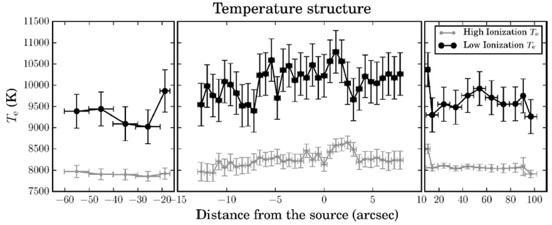
Fig. 4 The low-ionization electron temperature corresponds to [N II] λ5755/λ6584; the high-ionization temperature was calculated using [O III] λ4363/λ5007.
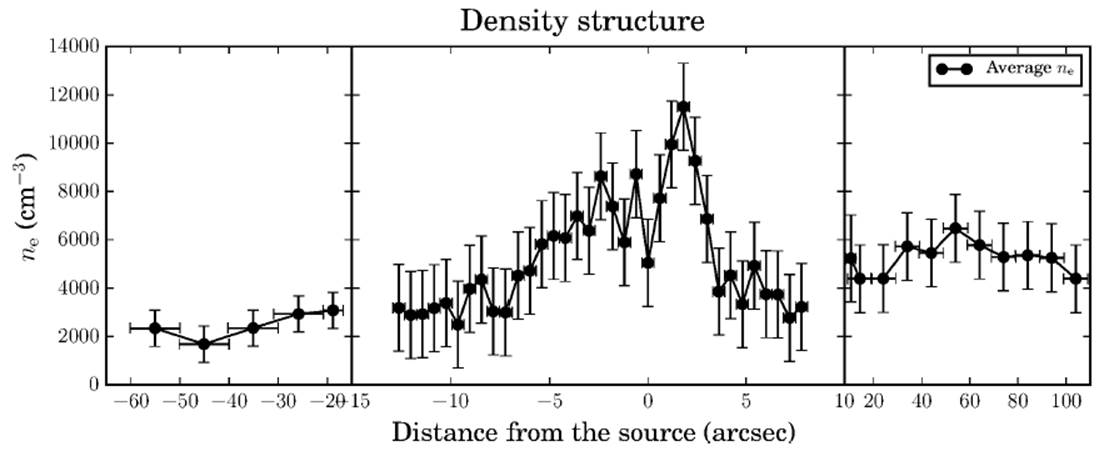
Fig. 5 The electron density shown is an average of the [S II] λλ 6716/6731 and [Cl III] λλ 5518/5538 diagnostics.
The physical conditions reported here were obtained using PyNeb (Luridiana et al. 2015), by identifying the intersection of the corresponding temperature and density diagnostics. Our results for the North and South zones away from the shock agree with previous determinations made by Rubin et al. (2003), Esteban et al. (2004) and Mesa-Delgado et al. (2009a). In the case of the shocked spectra, our results overlap with the upper limit reported for the [N II] electron temperature by Esteban et al. (2004), and also with the lower limits for the [ClIII] and [O II] densities. However, our reported [O III] temperature is about 300 K higher. We attribute this difference to the fact that we are not observing the same volume of gas; also, differences in calibration and the extinction law used may cause these minor disparities. However, this does not have major implications on the chemical abundances since the dependency of an emission line intensity on ne is minimal; moreover, for recombination lines the dependency on temperature is negligible.
We computed the total abundance for oxygen in two ways: from collisionally excited lines (CELs) and recombination lines (RLs). The abundance from CELs, OCEL, is the sum of the O+ and O2+ ionic abundances, obtained from [O III] λ5007 and [OII] λ3726+29 respectively. For the RL oxygen abundance we used multiplet 1 of O II to determine O2+/H+. The intensity of multiplet 1 of O II is the sum of eight lines, of which we only detected four blended in pairs as λλ4639 + 42 and λλ4649 + 51. The total intensity was estimated considering the dependence on density and temperature of the lines, according to the work of Peimbert & Peimbert (2010). The effective recombination coeficients were taken from Storey (1994) for case B, assuming ne = 10, 000 cm−3. Although O I lines are present in our spectra, they are contaminated by telluric emission, making them unreliable for calculating O+. To account for O+ we assumed the following relation between O+ and O2+:
Esteban et al. (2004) also favor this procedure. Oxygen abundances derived from RLs and CELs are presented in Figure 6. While small, there is a significant difference between the oxygen abundance near the apex of HH202-S compared with the surrounding -presumed static- gas; it is also evident from Figure 6 that OCEL and ORL are irreconcilable in the line of sight of the shock.
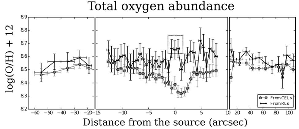
Fig. 6 Total O/H ratio computed using CELs and O II RLs (see text). Note that the difference is maximum at the apex of the shock.
It is known that oxygen is present in interstellar dust grains in the form of water ice and metallic compounds such as FeO, CaO and MgO. Theoretical and empirical studies have shown that dust can be destroyed by grain-grain collisions in interstellar shocks -a process known as sputtering- thus reincorporating refractory elements into the diffuse gas. However, these studies have been carried out mostly for molecular clouds (see, for example Podio et al. 2009 and references therein) and supernova remnants (Gall et al. 2014; Mouri & Taniguchi 2000). The dust composition in H II regions is known to be different from that found for molecular clouds due to photo-evaporation of ice molecules by UV radiation; in any case the relation between dust destruction and shock velocity is not entirely clear. The only work studying destruction in a Herbig-Haro object within an H II region and its effect on oxygen was that of Mesa-Delgado et al. (2009a) who also examined HH202-S and found an increase in the oxygen, iron and magnesium abundance at the shock; they showed the presence of dust destruction in the aftermath of moderate shockwaves. This effect is also present in our observations.
There has been a long debate on the magnitude of thermal inhomogeneities in H II regions and on their effect on the determination of chemical abundances (Peimbert & Costero 1969; Simón-Díaz & Stasinska 2011; Peña-Guerrero et al. 2012). Regardless of the typical effect on HII regions, an interstellar shock is clearly a case where non-negligible temperature variations are expected. Given that RLs are not affected by temperature variations to the same extent as CELs, we favored abundance determinations done with RLs for the analysis of dust destruction.
4. Analysis from combined spectra
In order to enhance the signal to noise ratio and reduce the bias produced by measuring very weak lines we decided to combine the three spectra with the highest Fe and O abundance (the ones with maximum dust destruction), which we will call the strongly shocked zone (SS), represented in Figure 6 with a box at the zero mark. To represent the static gas we chose two regions: one averaging 4 windows 20 arcseconds south of HH 202-S (South Zone), and one averaging 4 regions 20 arcseconds north of HH 202-S (North Zone). Finally, we also combined the spectra of four weakly shocked zones (WS). The resulting spectra were thoroughly studied to derive most of the conclusions of this work.
The dereddened fluxes for Hβ corresponding to the extinction law of Costero & Peimbert (1970) are presented at the bottom of Table 3.
Table 3 List of emission line intensities for HH202-s and the Orion nebulaa
| North zone | WS zone | SS zone | South zone | |||||||
| λ | Ion | f(λ) | I | % err | I | % err | I | % err | I | % err |
| 3587 | He I | 0.214 | 0.133 | 13 | 0.217 | 15 | 0.118 | 26 | 0.160 | 18 |
| 3614 | He I | 0.209 | 0.261 | 9 | … | … | 0.377 | 15 | 0.259 | 14 |
| 3634 | He I | 0.206 | 0.255 | 9 | 0.262 | 13 | … | … | 0.282 | 13 |
| 3676 | H 22 | 0.199 | 0.448 | 7 | … | … | … | … | … | … |
| 3679 | H 21 | 0.198 | 0.530 | 6 | 0.517 | 9 | 0.491 | 13 | 0.479 | 10 |
| 3683 | H 20 | 0.198 | 0.556 | 6 | 0.530 | 9 | 0.564 | 12 | 0.520 | 10 |
| 3687 | H 19 | 0.197 | 0.662 | 6 | 0.621 | 9 | 0.666 | 11 | 0.616 | 9 |
| 3692 | H 18 | 0.196 | 0.815 | 5 | 0.751 | 8 | 0.805 | 10 | 0.763 | 8 |
| 3697 | H 17 | 0.195 | 0.948 | 5 | 0.901 | 7 | 0.886 | 10 | 0.900 | 7 |
| 3704 | H 16 | 0.194 | 1.539 | 4 | 1.518 | 6 | 1.522 | 7 | 1.524 | 6 |
| 3712 | H 15 | 0.192 | 1.402 | 4 | 1.363 | 6 | 1.413 | 8 | 1.370 | 6 |
| 3722 | H 14 + [S II] | 0.190 | 0.628 | 6 | 1.619 | 5 | 1.823 | 7 | 1.470 | 6 |
| 3726 | [O II] | 0.190 | 85.732 | 1 | 60.557 | 1 | 66.532 | 1 | 63.628 | 1 |
| 3729 | [O II] | 0.189 | 52.546 | 1 | 29.413 | 2 | 29.748 | 2 | 28.685 | 2 |
| 3734 | H 13 | 0.189 | 2.348 | 3 | 2.119 | 5 | 2.092 | 7 | 2.229 | 5 |
| 3750 | H 12 | 0.186 | 3.086 | 3 | 3.118 | 4 | 3.093 | 6 | 3.070 | 4 |
| 3770 | H 11 | 0.182 | 3.952 | 3 | 3.958 | 4 | 3.923 | 5 | 3.917 | 4 |
| 3798 | H 10 | 0.177 | 5.218 | 2 | 5.236 | 3 | 5.188 | 4 | 5.156 | 3 |
| 3820 | He I | 0.174 | 1.066 | 5 | 1.097 | 7 | 1.073 | 9 | 1.095 | 7 |
| 3836 | H 9 | 0.171 | 7.329 | 2 | 7.208 | 3 | 7.303 | 4 | 7.272 | 3 |
| 3856 | Si II | 0.167 | … | … | 0.283 | 13 | 0.297 | 16 | 0.185 | 16 |
| 3863 | Si II | 0.166 | … | … | … | 0.175 | 21 | … | … | |
| 3869 | [Ne III] | 0.165 | 9.656 | 2 | 10.583 | 2 | 8.960 | 3 | 13.841 | 2 |
| 3889 | H 8 + He I | 0.162 | 17.338 | 1 | 15.693 | 2 | 15.250 | 3 | 16.300 | 2 |
| 3919 | C II? | 0.156 | 0.115 | 13 | 0.162 | 17 | 0.186 | 20 | 0.146 | 18 |
| 3927 | He I | 0.155 | 0.096 | 15 | 0.122 | 19 | 0.107 | 27 | 0.086 | 24 |
| 3933 | O I | 0.154 | … | … | 0.099 | 21 | 0.249 | 18 | … | … |
| 3970 | [Ne III] + H 7 | 0.148 | 20.435 | 1 | 20.452 | 2 | 19.940 | 2 | 21.698 | 2 |
| 3993 | [Ni II] | 0.144 | … | … | … | … | 0.063 | 35 | … | … |
| 4009 | He I | 0.141 | 0.288 | 10 | 0.492 | 11 | 0.661 | 12 | 0.288 | 16 |
| 4026 | He I | 0.138 | 1.974 | 3 | 2.119 | 5 | 2.038 | 6 | 2.091 | 5 |
| 4069 | [S II] | 0.130 | 1.255 | 4 | 2.454 | 4 | 4.200 | 4 | 1.642 | 5 |
| 4076 | [S II] | 0.129 | 0.445 | 7 | 0.928 | 7 | 1.548 | 7 | 0.608 | 9 |
| 4102 | Hδ | 0.125 | 26.277 | 1 | 26.249 | 2 | 25.970 | 2 | 26.779 | 2 |
| 4114 | [Fe II] | 0.122 | … | … | … | 0.119 | 25 | … | … | |
| 4121 | He I | 0.121 | 0.180 | 11 | 0.226 | 14 | 0.220 | 19 | 0.209 | 15 |
| 4131 | O II | 0.119 | … | … | … | … | … | 0.037 | 36 | |
| 4144 | He I | 0.117 | 0.238 | 9 | 0.259 | 13 | 0.256 | 17 | 0.269 | 13 |
| 4155 | O II + N II | 0.116 | … | … | … | … | 0.058 | 36 | 0.051 | 30 |
| 4169 | O II | 0.113 | 0.039 | 22 | … | … | 0.027 | 53 | 0.043 | 33 |
| 4178 | [Fe II] | 0.112 | … | … | … | … | 0.076 | 31 | … | … |
| 4244 | [Fe II]+[Fe III] | 0.100 | 0.327 | 8 | 0.133 | 18 | 0.432 | 13 | … | … |
| 4249 | [Ni II] + [Fe II] | 0.099 | … | … | 0.232 | 14 | 0.223 | 18 | 0.183 | 16 |
| 4267 | C II | 0.096 | 0.234 | 9 | 0.209 | 14 | 0.213 | 19 | 0.216 | 15 |
| 4277 | [Fe II] | 0.095 | 0.045 | 21 | 0.064 | 26 | 0.215 | 19 | 0.041 | 34 |
| 4287 | [Fe II] | 0.093 | 0.112 | 13 | 0.108 | 20 | 0.449 | 13 | 0.082 | 24 |
| 4320 | [Fe II] | 0.088 | … | … | … | … | 0.153 | 22 | … | … |
| 4326 | [Ni II] | 0.086 | … | … | 0.123 | 18 | 0.274 | 16 | 0.053 | 29 |
| 4340 | Hγ | 0.084 | 46.866 | 1 | 47.007 | 1 | 46.735 | 2 | 46.622 | 1 |
| 4353 | [Fe II] | 0.082 | … | … | … | … | 0.119 | 25 | … | … |
| 4363 | [O III] | 0.080 | 0.829 | 5 | 1.033 | 6 | 0.903 | 9 | 1.060 | 7 |
| 4388 | He I | 0.076 | 0.515 | 7 | 0.613 | 9 | 0.583 | 12 | 0.586 | 9 |
| 4415 | O II | 0.072 | 0.146 | 11 | 0.235 | 13 | 0.607 | 11 | 0.129 | 19 |
| 4438 | He I | 0.068 | 0.051 | 19 | 0.059 | 26 | 0.050 | 38 | 0.065 | 26 |
| 4452 | [Fe II] | 0.065 | … | … | 0.058 | 27 | 0.157 | 21 | 0.032 | 37 |
| 4458 | [Fe II] | 0.062 | … | … | 0.050 | 29 | 0.136 | 23 | … | … |
| 4471 | He I | 0.055 | 4.350 | 2 | 4.708 | 3 | 4.494 | 4 | 4.594 | 3 |
| 4515 | [Fe II] | 0.046 | … | … | … | … | 0.040 | 42 | … | … |
| 4571 | Mg I] | 0.044 | … | … | … | … | 0.233 | 17 | … | … |
| 4581 | [Cr III] | 0.042 | … | … | … | … | 0.037 | 44 | … | … |
| 4595 | [Co IV] ? | 0.042 | … | … | 0.060 | 26 | 0.090 | 28 | 0.018 | 49 |
| 4607 | [Fe III] | 0.040 | 0.049 | 19 | 0.308 | 11 | 0.597 | 11 | 0.051 | 29 |
| 4630 | N II | 0.036 | 0.027 | 26 | 0.029 | 38 | 0.031 | 48 | 0.033 | 36 |
| 4642 | O II | 0.035 | 0.109 | 13 | 0.132 | 17 | 0.162 | 21 | 0.145 | 17 |
| 4650 | O II | 0.033 | 0.102 | 13 | 0.143 | 17 | 0.134 | 23 | 0.137 | 18 |
| 4658 | [Fe III] | 0.032 | 0.793 | 5 | 4.896 | 3 | 9.533 | 3 | 0.711 | 8 |
| 4665 | [Fe III] | 0.031 | … | … | 0.198 | 14 | 0.444 | 13 | 0.018 | 49 |
| 4701 | [Fe III] | 0.025 | 0.219 | 9 | 1.716 | 5 | 3.311 | 5 | 0.220 | 14 |
| 4711 | [Ar IV]+He I | 0.023 | 0.531 | 6 | 0.570 | 8 | 0.546 | 11 | 0.645 | 8 |
| 4728 | [Fe II] | 0.021 | … | … | … | … | 0.103 | 26 | … | … |
| 4734 | [Fe III] | 0.020 | 0.072 | 16 | 0.781 | 7 | 1.502 | 7 | 0.080 | 23 |
| 4740 | [Ar IV] | 0.019 | 0.021 | 29 | … | … | … | … | … | … |
| 4755 | [Fe III] | 0.017 | 0.142 | 11 | 0.937 | 7 | 1.753 | 6 | 0.140 | 17 |
| 4770 | [Fe III] | 0.014 | 0.070 | 16 | 0.600 | 8 | 1.165 | 8 | 0.071 | 25 |
| 4779 | [Fe III] | 0.013 | 0.044 | 20 | 0.383 | 10 | 0.808 | 9 | 0.043 | 31 |
| 4797 | Cl I | 0.010 | 0.049 | 19 | … | … | 0.069 | 32 | … | … |
| 4800 | O I? | 0.009 | … | … | 0.076 | 23 | … | … | 0.056 | 28 |
| 4815 | [Fe II] | 0.007 | 0.065 | 17 | 0.104 | 19 | 0.328 | 15 | 0.047 | 30 |
| 4861 | Hβ | 0.000 | 98.818 | 1 | 100.004 | 1 | 99.705 | 1 | 98.332 | 1 |
| 4874 | [Fe II] | 0.000 | … | … | … | … | 0.108 | 25 | … | … |
| 4881 | [Fe III] | -0.001 | 0.276 | 8 | 2.625 | 4 | 5.003 | 4 | 0.292 | 12 |
| 4890 | [Fe II] | -0.001 | 0.033 | 23 | 0.070 | 24 | 0.229 | 17 | 0.022 | 43 |
| 4895 | [Fe II]+[Cr III] | -0.001 | 0.047 | 19 | … | … | … | … | … | … |
| 4905 | [Fe II] | -0.001 | 0.021 | 29 | 0.078 | 22 | 0.145 | 22 | 0.029 | 38 |
| 4922 | He I | -0.002 | 1.205 | 4 | 1.325 | 6 | 1.307 | 8 | 1.272 | 6 |
| 4931 | [Fe III] | -0.002 | 0.065 | 16 | 0.262 | 12 | 0.523 | 11 | 0.053 | 28 |
| 4959 | [O III] | -0.004 | 85.528 | 1 | 96.013 | 1 | 79.275 | 1 | 101.927 | 1 |
| 4987 | [Fe III] | -0.006 | 0.091 | 14 | 0.448 | 9 | 0.916 | 9 | 0.050 | 29 |
| 5007 | [O III] | -0.007 | 253.745 | 1 | 283.142 | 1 | 238.115 | 1 | 304.533 | 1 |
| 5016 | He I | -0.008 | 2.360 | 3 | 2.501 | 4 | 2.347 | 6 | 2.456 | 4 |
| 5041 | Si II | -0.010 | 0.104 | 13 | 0.143 | 16 | … | … | 0.064 | 26 |
| 5048 | He I | -0.010 | 0.240 | 10 | 0.253 | 16 | 0.240 | 22 | 0.250 | 16 |
| 5056 | Si II | -0.011 | 0.181 | 10 | 0.236 | 13 | 0.253 | 16 | 0.139 | 17 |
| 5085 | [Fe III] | -0.014 | … | … | … | … | 0.288 | 15 | … | … |
| 5112 | [Fe II] | -0.017 | 0.031 | 24 | 0.028 | 37 | 0.157 | 21 | … | … |
| 5147 | O II | -0.020 | 0.044 | 20 | 0.039 | 31 | … | … | 0.034 | 35 |
| 5159 | [Fe II] | -0.022 | 0.097 | 13 | 0.280 | 12 | 1.000 | 8 | 0.067 | 25 |
| 5192 | [Ar III] | -0.026 | 0.046 | 19 | 0.062 | 25 | 0.042 | 40 | 0.056 | 27 |
| 5198 | [N I] | -0.027 | 0.518 | 6 | 0.218 | 13 | 0.230 | 17 | 0.293 | 12 |
| 5220 | [Fe II] | -0.029 | … | … | 0.029 | 36 | 0.096 | 26 | … | … |
| 5262 | [Fe II] | -0.035 | 0.085 | 14 | 0.120 | 18 | 0.457 | 12 | 0.046 | 30 |
| 5270 | [Fe III] | -0.036 | 0.409 | 7 | 2.918 | 4 | 5.721 | 4 | 0.387 | 10 |
| 5299 | O I | -0.040 | 0.039 | 21 | … | … | 0.070 | 31 | 0.027 | 39 |
| 5334 | [Fe II] | -0.045 | … | … | 0.067 | 24 | 0.243 | 16 | 0.018 | 48 |
| 5376 | [Fe II] | -0.052 | … | … | 0.029 | 36 | 0.164 | 15 | … | … |
| 5412 | [Fe III] | -0.058 | 0.018 | 30 | 0.276 | 12 | 0.583 | 8 | 0.018 | 33 |
| 5433 | [Fe II] | -0.061 | … | … | … | … | 0.077 | 21 | 0.017 | 35 |
| 5455 | [Cr III] | -0.064 | … | … | … | … | 0.067 | 23 | 0.009 | 46 |
| 5472 | [Cr III] | -0.067 | … | … | … | … | 0.090 | 20 | … | … |
| 5485 | [Cr III] | -0.069 | … | … | … | … | 0.050 | 27 | … | … |
| 5496 | [Fe II] | -0.071 | … | … | … | … | 0.036 | 31 | … | … |
| 5507 | [Cr III] | -0.073 | … | … | … | … | 0.137 | 16 | … | … |
| 5513 | O I | -0.075 | 0.032 | 23 | … | … | … | … | 0.022 | 30 |
| 5518 | [Cl III] | -0.075 | 0.466 | 6 | 0.376 | 10 | 0.375 | 10 | 0.416 | 7 |
| 5527 | [Fe II] | -0.077 | … | … | 0.061 | 25 | 0.267 | 11 | 0.015 | 37 |
| 5538 | [Cl III] | -0.079 | 0.468 | 6 | 0.527 | 8 | 0.534 | 8 | 0.547 | 6 |
| 5552 | [Cr III] | -0.081 | … | … | 0.115 | 18 | 0.260 | 12 | … | … |
| 5555 | O I | -0.082 | 0.041 | 20 | … | … | … | 0.029 | 26 | |
| 5667 | N II | -0.103 | 0.021 | 28 | … | … | 0.037 | 30 | 0.028 | 27 |
| 5680 | N II | -0.105 | … | … | … | … | 0.036 | 31 | 0.034 | 24 |
| 5715 | [Cr III] | -0.106 | … | … | … | … | 0.124 | 17 | … | … |
| 5747 | [Fe II] | -0.111 | … | … | … | … | 0.048 | 26 | … | … |
| 5755 | [N II] | -0.120 | 0.735 | 5 | 0.965 | 6 | 1.302 | 5 | 0.790 | 5 |
| 5867 | O I | -0.130 | … | … | … | … | … | … | 0.037 | 23 |
| 5876 | He I | -0.144 | 12.920 | 1 | 13.351 | 2 | 13.535 | 2 | 13.614 | 2 |
| 5932 | N II | -0.155 | … | … | … | … | … | … | 0.018 | 33 |
| 5942 | N II | -0.157 | … | … | … | … | … | … | 0.026 | 27 |
| 5958 | Si II + O I | -0.160 | … | … | … | … | 0.153 | 15 | 0.076 | 16 |
| 5979 | Si II | -0.165 | … | … | … | … | 0.220 | 12 | 0.086 | 15 |
| 6000 | [Ni III] | -0.169 | … | … | … | … | 0.122 | 16 | 0.013 | 38 |
| 6046 | O I | -0.179 | … | … | … | … | 0.077 | 20 | 0.077 | 15 |
| 6312 | [S III] | -0.234 | 1.560 | 3 | 1.966 | 4 | 1.935 | 4 | 1.760 | 3 |
| 6347 | Si II | -0.242 | … | … | 0.251 | 11 | 0.300 | 10 | 0.132 | 12 |
| 6371 | Si II | -0.247 | … | … | 0.129 | 16 | 0.146 | 14 | 0.067 | 16 |
| 6400 | [Ni III] | -0.253 | … | … | 0.055 | 24 | 0.083 | 19 | 0.014 | 35 |
| 6440 | [Fe II] | -0.261 | … | … | … | … | 0.052 | 24 | … | … |
| 6534 | [Ni III] | -0.281 | … | … | … | … | 0.178 | 13 | … | … |
| 6548 | [N II] | -0.284 | 18.984 | 1 | 18.795 | 2 | 23.987 | 1 | 16.555 | 1 |
| 6563 | Hα | -0.287 | 288.294 | 1 | 289.239 | 1 | 288.392 | 1 | 288.675 | 1 |
| 6578 | C II | -0.290 | 0.337 | 7 | … | … | … | … | 0.281 | 8 |
| 6583 | [N II] | -0.291 | 56.261 | 1 | 57.606 | 1 | 72.984 | 1 | 49.607 | 1 |
| 6669 | [Ni II] | -0.308 | … | … | … | … | 0.101 | 17 | 0.020 | 29 |
| 6678 | He I | -0.310 | 3.375 | 2 | 3.658 | 3 | 3.516 | 3 | 3.590 | 2 |
| 6716 | [S II] | -0.318 | 5.154 | 2 | 3.347 | 3 | 4.480 | 3 | 2.918 | 3 |
| 6731 | [S II] | -0.321 | 7.142 | 2 | 6.040 | 2 | 8.430 | 2 | 4.990 | 2 |
| 6797 | [Ni III] | -0.334 | … | … | … | … | 0.022 | 36 | … | … |
| 6946 | [Ni III] | -0.364 | … | … | 0.029 | 32 | … | … | … | … |
| 7002 | O I | -0.375 | 0.100 | 11 | … | … | 0.077 | 19 | 0.063 | 16 |
| 7065 | He I | -0.388 | 4.297 | 2 | 4.802 | 3 | 4.582 | 3 | 5.536 | 2 |
| 7110 | O II? | -0.396 | … | … | … | … | 0.046 | 24 | 0.044 | 19 |
| 7136 | [Ar III] | -0.401 | 11.611 | 1 | 13.700 | 2 | 12.382 | 2 | 13.967 | 1 |
| 7155 | [Fe II] | -0.405 | 0.059 | 15 | 0.304 | 10 | 1.436 | 4 | 0.050 | 17 |
| 7161 | He I | -0.410 | … | … | … | … | … | … | 0.018 | 29 |
| 7231 | C II | -0.419 | 0.063 | 14 | 0.093 | 17 | 0.078 | 18 | 0.078 | 14 |
| 7236 | C II | -0.421 | 0.157 | 9 | 0.134 | 14 | 0.097 | 16 | 0.148 | 10 |
| 7254 | O I | -0.424 | … | … | … | … | 0.111 | 15 | 0.081 | 14 |
| 7281 | He I | -0.429 | 0.554 | 5 | 0.636 | 7 | 0.607 | 7 | 0.621 | 5 |
| 7291 | [Ca II] | -0.431 | … | … | 0.138 | 14 | 0.572 | 7 | … | … |
| 7298 | He I | -0.432 | 0.032 | 20 | … | … | … | … | 0.035 | 21 |
| 7320 | [O II] | -0.436 | 3.673 | 2 | 6.784 | 2 | 9.330 | 2 | 5.244 | 2 |
| 7330 | [O II] | -0.438 | 2.977 | 2 | 5.694 | 2 | 7.656 | 2 | 4.305 | 2 |
| 7341 | Ca I | -0.440 | … | … | … | … | … | … | 0.042 | 19 |
| 7370 | Ca I | -.445 | … | … | … | … | … | … | 0.025 | 24 |
| 7378 | [Ni II] | -0.447 | 0.080 | 12 | … | … | 1.297 | 5 | 0.067 | 15 |
| 7388 | [Fe II] | -0.449 | … | … | 0.079 | 18 | 0.285 | 10 | … | … |
| 7402 | Ca II | -0.450 | … | … | … | … | … | … | 0.018 | 29 |
| 7412 | [Ni II] | -0.453 | … | … | … | … | 0.137 | 14 | 0.019 | 28 |
| 7424 | Ca I | -0.456 | … | … | … | … | … | … | 0.007 | 47 |
| 7443 | S I | -0.459 | … | … | … | … | … | … | 0.017 | 29 |
| 7453 | [Fe II] | -0.460 | … | … | 0.091 | 17 | 0.442 | 8 | 0.015 | 32 |
| I(Hβ)b | 8.96E-012 | 1.55E-012 | 1.49E-012 | 1.80E-011 | ||||||
| C(Hβ) | 0.35 | 0.36 | 0.37 | 0.35 | ||||||
| EWabs(Hβ) | 3.8 | 6.6 | 7.0 | 4.4 | ||||||
aEmission lines corrected for reddening, underlying absorption and normalized with respect to the entire Balmer decrement.
bDereddened flux for Hβ in units of erg cm−2 s−1. The North and South zones are the sum of four 50-pixel long spectra from the Orion Nebula. The weakly and strongly shocked zones are the sum of four and three 3 pixel long spectra respectively covering HH202-S (see text).
The emission line intensities for the four combined spectra covering the northern and southern zones of the Orion Nebula as well as HH202-S are presented in Table 3 in Columns 4-11. Column 1 shows the laboratory wavelength λ for air; Column 2 presents the identification of each line based on the work by Esteban et al. (2004) and the Atomic Line List v2.045; Column 3 presents the value of f (λ) for each line. Overall, we identified 169 different emission lines in our combined spectra; the Strongly Shocked Zone had the most emission lines, with 159, including several additional Cr and Fe lines.
From Table 3 we can ascertain that dust is being destroyed by the shock front. Comparing the intensity of the iron emission lines in the strongly shocked zone with an average for the North and South zones we find that all of them are brighter at the apex of HH202-S; particularly, [Fe II] λ7155 is 26 times more intense at the shock and [Fe III] λ4658 is 13 times brighter. The increase in the gaseous abundance at the shock is due to the incorporation of this iron by the destruction of dust grains.
We computed diagnostics for Te and ne using PyNeb. For high ionization we used: [OIII] λ4363/λ5007, and [ArIII] λ5192/λ7136 for Te; and [ClIII] λ5518/λ5538 for ne. For low ionization we computed: [NII] λ5755/λλ6548 + 84, [O II] λλ3726 + 29 /λλ7319 + 30, [S II] λλ4069 + 76/λλ6716+31 for Te; and [OII] λ3726/λ3729, [S II] λ6716/λ6731 for ne. These diagnostics are presented in Figure 7. The high ionization temperature and density were determined from the intersection of the [O III] and [Cl III] diagnostics. For low ionization, the physical conditions were determined graphically from the available diagnostics (see the aforementioned figures) by establishing the midpoint between the [N II], [O II], and [S II] lines. Table 4 presents the specific physical conditions for each diagnostic as well as the adopted Te and ne.
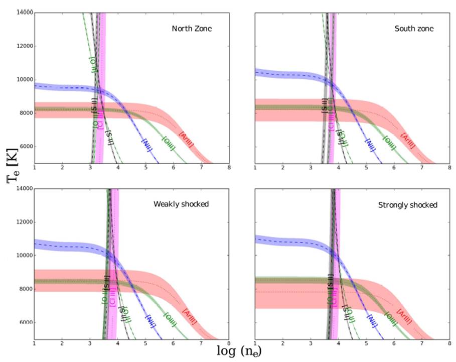
Fig. 7 Electron temperature and density diagnostics for the four analyzed zones of the Orion Nebula.
Table 4 Physical conditions from combined spectra
| Diagnostic | North Zone | South Zone | WS Zone | SS Zone | |
| Te (K) | [O III] | 8210 ± 120 | 8320 ± 170 | 8410 ± 160 | 8490 ± 220 |
| [Ar III] | 8200 ± 440 | 8220 ± 650 | 8530 ± 670 | 7830 ± 890 | |
| [N II] | 9370 ± 200 | 9800 ± 300 | 10060 ± 300 | 10125 ± 240 | |
| [S II] | 10180 ± 400 | 11680 ± 800 | 19920 ±2500 1500 | 17710 ± 1000 | |
| [O II] | 13120 ± 600 | 14700 ± 900 | 23150 ± 1500 | 21400 ± 2200 | |
| Adopted HI | 8210 ± 150 | 8320 ± 200 | 8410 ± 200 | 8490 ± 300 | |
| Adopted LI | 9500 ± 250 | 9780 ± 300 | 10230 ± 300 | 10260 ± 350 | |
| ne (cm−3) | [Cl III] | 2500 ± 1100 | 5980+2700 −1900 | 7200+5100 −3000 | 7550+5300 −3000 |
| [O II] | 1860 ± 110 | 5720 ± 800 | 4230 ± 500 | 6300 ± 900 | |
| [S II] | 1530 ± 200 | 3500 ± 600 | 4590 ± 1100 | 5800 ± 1500 | |
| Adopted HI | 2500 ± 1000 | 5980 ± 2000 | 7200 ± 3000 | 7550 ± 3000 | |
| Adopted LI | 1800 ± 200 | 4750 ± 500 | 4250 ± 600 | 6100 ± 900 | |
We followed the formalism developed by Peimbert (1967) to account for thermal inhomogeneities in the temperature structure of the nebula along the line of sight. This approach establishes an average temperature, T0 and the mean square temperature inhomogeneities, t2, defined as:
For the case of O2+ we can derive the following Equation (Peimbert et al. 2004):
A similar equation can be derived for the T 0 of the low-ionization species.
Once T0 and 2 have been determined, Equation 4 is used to calculate the O2+ abundance (Peimbert & Costero 1969; Esteban et al. 2004).
4.1. Chemical Composition
Ionic abundances were derived for O+, O2+, N+, Ne2+, S+, S2+, Cl2+, Ar2+, Fe+, Fe2+, and Ni2+, from CELs using PyNeb. Just as in the previous section, oxygen abundances were computed using recombination lines from those of Multiplet 1. The Fe+ abundance was estimated using only [Fe II] λ7155 as it is the only line available in our observed range not affected by fluorescence; meanwhile, the Fe2+ abundance was determined using the emission of [Fe III] λ4734, λ4755 and λ4881, since these lines are not contaminated by emission of other ions.
The He+ abundance was calculated from recombination lines using HELIO13, a
software package described in Peimbert et al.
(2012) that uses a maximum likelihood method to perform a
simultaneous fitting of ne , τ3889 , the
He+ abundance, t2, and T
0. We present the final adopted value of t2 for each
region in Table 5. In Table 7, we present the ionic abundances
assuming both homogeneous and inhomogeneous temperature distributions: as
mentioned in § 3 we prefer abundance determinations with t2
Table 5 t2 Values
| North Zone | South Zone | WS Zone | SS Zone |
| 0.014 ± 0.005 | 0.022 ± 0.004 | 0.024 ± 0.006 | 0.039 ± 0.006 |
Table 6 Oxygen depletion factors
| Method | Value | Reference |
| Fe/O ratio | −0.12 ± 0.04 | This work |
| −0.11 + 0.11 − 0.14 | Mesa-Delgado et al. (2009a) | |
| Comparison with Orion stars | −0.18 ± 0.05 | This work |
| −0.17 ± 0.06 | Mesa-Delgado et al. (2009a) | |
| Molecular composition | −0.10 ± 0.04 | Esteban et al. (1998); Mesa-Delgado et al. (2009a) |
Table 7 Ionic abundances
| Ion | North zone | South zone | WS zone | SS zone | ||||
| t2 = 0.00 | t2 = 0.014 | t2 = 0.00 | t2 = 0.022 | t2 = 0.00 | t2 = 0.024 | t2 = 0.024 | t2 = 0.039 | |
| Ar2+ | 6.25 ± 0.02 | 6.34 ± 0.03 | 6.31 ± 0.03 | 6.45 ± 0.03 | 6.30 ± 0.03 | 6.44 ± 0.04 | 6.23 ± 0.04 | 6.48 ± 0.04 |
| Cl2+ | 5.08 ± 0.04 | 5.19 ± 0.05 | 5.11 ± 0.03 | 5.27 ± 0.06 | 5.08 ± 0.03 | 5.25 ± 0.06 | 5.06 ± 0.03 | 5.35 ± 0.07 |
| Fe+ | 4.72: | 4.77: | 4.59: | 4.66: | 5.34: | 5.41: | 6.00: | 6.12: |
| Fe2+ | 5.60 ± 0.04 | 5.65 ± 0.05 | 5.52 ± 0.06 | 5.60 ± 0.06 | 6.38 ± 0.03 | 6.46 ± 0.03 | 6.64 ± 0.04 | 6.77 ± 0.05 |
| N+ | 7.13 ± 0.03 | 7.18 ± 0.03 | 7.05 ± 0.03 | 7.12 ± 0.04 | 7.05 ± 0.03 | 7.12 ± 0.03 | 7.17 ± 0.04 | 7.29 ± 0.04 |
| Ne2+ | 7.42 ± 0.03 | 7.54 ± 0.05 | 7.55 ± 0.04 | 7.73 ± 0.06 | 7.41 ± 0.05 | 7.61 ± 0.05 | 7.31 ± 0.06 | 7.63 ± 0.07 |
| Ni2+ | … | … | 4.46 ± 0.10 | 4.60 ± 0.11 | 4.99 ± 0.07 | 5.13 ± 0.07 | 5.24 ± 0.06 | 5.43 ± 0.07 |
| O+ | 7.91 ± 0.02 | 7.97 ± 0.04 | 7.80 ± 0.03 | 7.90 ± 0.04 | 7.69 ± 0.02 | 7.79 ± 0.03 | 7.79 ± 0.03 | 7.95 ± 0.05 |
| O2+ | 8.29 ± 0.02 | 8.38 ± 0.03 | 8.34 ± 0.04 | 8.49 ± 0.05 | 8.30 ± 0.03 | 8.47 ± 0.04 | 8.20 ± 0.04 | 8.50 ± 0.05 |
|
|
8.38 ± 0.04 | 8.49 ± 0.05 | 8.47 ± 0.05 | 8.51 ± 0.06 | ||||
| S+ | 5.70 ± 0.02 | 5.75 ± 0.03 | 5.63 ± 0.04 | 5.70 ± 0.06 | 5.62 ± 0.02 | 5.69 ± 0.03 | 5.84 ± 0.02 | 5.95 ± 0.05 |
| S2+ | 6.94 ± 0.05 | 7.06 ± 0.06 | 6.96 ± 0.06 | 7.14 ± 0.07 | 6.98 ± 0.06 | 7.18 ± 0.07 | 6.95 ± 0.07 | 7.27 ± 0.09 |
|
|
10.926 ± 0.004 | 10.922 ± 0.004 | 10.952 ± 0.006 | 10.936 ± 0.005 | 10.951 ± 0.006 | 10.940 ± 0.006 | 10.959 ± 0.007 | 10.922 ± 0.008 |
In order to calculate total abundances, we have to consider the contribution from unseen ions; this was done assuming a series of ionization correction factors (ICFs) from different sources. We do not expect this to be the case of oxygen, whose total abundance is simply the sum of O+ and O2+.
For nitrogen we used the classic ICF, to account for the presence of N2+:
The total neon abundance has a contribution from Ne2+, which we have taken in consideration using the ICF from Peimbert & Costero (1969):
Besides S+ and S2+, it is known that S3+ must be present in H II regions from the work of Stasinska (1978):
Helium has to be corrected for the presence He0; we did this using the ICF derived by Peimbert et al. (1992):
However, as Delgado-Inglada et al. (2014) point out, this result has to be taken with reservation, since the population of helium ions depends on the effective temperature of the ionizing stars, and that of sulfur on the ionization parameter.
We observed [Cl III] emission lines in our spectra. However, Cl+ and possibly Cl3+ also contribute to the total chlorine abundance. Delgado-Inglada et al. (2014) proposed a ICF which, although intended for use in planetary nebulae, can be used in this case as it depends on the ionic fraction of oxygen and the observed abundance of Cl2+:
This expression is valid when the ionic fraction of oxygen -the term in square brackets- takes a value between 0.02 and 0.95.
It is known that Ar+ can contribute a significant fraction to the total abundance. For this work, we employed the ICF obtained by Delgado-Inglada et al. (2014) from Cloudy photoionization models, which depends only on the Ar2+ lines:
with
Uncertainties in the atomic data affect some ions more than others. Given the complex structure of Fe+ and Fe2+, the atomic data currently available does not yet represent a complete picture of this element; furthermore, it is known that many [Fe II] lines are affected by fluorescence. To compute the total iron abundance, Rodríguez & Rubin (2005) proposed two ICFs based on observations and photoionization models which require only [Fe III] lines. We decided to use their observational ICF since the one from the models produces results for the total iron abundance that would imply a complete destruction of interstellar dust grains (see § 5.1), something that is not expected in these observations, since we have substantial amounts of unshocked gas in front of and behind the shocked region. Also, this shock is not fast enough to be expected to destroy all the dust grains it encounters. Thus
Nickel poses similar problems as iron in that [Ni II] lines may be affected by fluorescence. Until recently, most studies have used an ICF for nickel based on the similarity of the ionization potentials of Fe+ and Ni+. Based on multiple observational data and photoionization models, Delgado-Inglada et al. (2016) derived two ICFs for Ni that required only [Ni III] lines. From Equation 6 of their paper -applicable when He2+ is not present- we have that:
We used [Ni III] λ4326, λ6000, and λ6401 to calculate the total abundance, since these lines are not contaminated by others in our spectra.
Total abundances are presented in Table 8 considering both a homogeneous (t2
Table 8 Total abundances
| Element | North zone | South zone | WS zone | SS zone | ||||
| t 2 = 0.00 | t 2 = 0.014 | t 2 = 0.00 | t 2 = 0.022 | t 2 = 0.00 | t 2 = 0.024 | t 2 = 0.00 | t 2 = 0.039 | |
| Ar | 6.31±0.2 0.52 | 6.41±0.2 0.52 | 6.40 ±0.2 0.52 | 6.55±0.2 0.52 | 6.40 ±0.2 0.52 | 6.56±0.2 0.52 | 6.28±0.2 0.52 | 6.58±0.2 0.52 |
| Cl | 5.22 ±0.06 0.14 | 5.32±0.06 0.14 | 5.26 ±0.06 0.14 | 5.42±0.06 0.14 | 5.24 ±0.06 0.14 | 5.42 ±0.06 0.14 | 5.19±0.06 0.14 | 5.50 ±0.06 0.14 |
| Fe | 5.95 ± 0.04 | 6.00 ± 0.06 | 5.91 ± 0.06 | 5.99 ± 0.08 | 6.78 ± 0.05 | 6.87 ± 0.05 | 7.00 ± 0.06 | 7.15 ± 0.07 |
| N | 7.67 ± 0.03 | 7.73 ± 0.05 | 7.71 ± 0.02 | 7.81 ± 0.06 | 7.76 ± 0.03 | 7.88 ± 0.05 | 7.71 ± 0.02 | 7.95 ± 0.06 |
| Ne | 7.57 ± 0.03 | 7.69 ± 0.04 | 7.66 ± 0.05 | 7.83 ± 0.06 | 7.51 ± 0.04 | 7.69 ± 0.05 | 7.45 ± 0.07 | 7.74 ± 0.08 |
| Ni | … | … | 4.72 ± 0.03 | 4.88 ± 0.04 | 5.28 ± 0.04 | 5.45 ± 0. | 5.45 ± 0.04 | 5.69 ± 0.04 |
| OCEL | 8.44 ± 0.02 | 8.52 ± 0.02 | 8.45 ± 0.03 | 8.59 ± 0.04 | 8.39 ± 0.03 | 8.56 ± 0.03 | 8.34 ± 0.03 | 8.61 ± 0.04 |
| ORL | 8.53 ± 0.04 | 8.60 ± 0.05 | 8.57 ± 0.05 | 8.65 ± 0.06 | ||||
| S | 6.98 ± 0.04 | 7.09 ± 0.05 | 6.98 ± 0.06 | 7.16 ± 0.07 | 7.00 ± 0.06 | 7.19 ± 0.07 | 7.00 ± 0.07 | 7.30 ± 0.08 |
| HeRL | 10.950 ± 0.005 | 10.94 ± 0.01 | 10.972 ± 0.007 | 10.96 ± 0.01 | 10.973 ± 0.007 | 10.96 ± 0.01 | 10.990 ± 0.009 | 10.95 ± 0.01 |
5. Discussion
The results obtained here for Te and Ne for the North and South zones agree with previous determinations by Esteban et al. (2004) and Rubin et al. (2003). For the shocked zones we must compare our results directly with those of Mesa-Delgado et al. (2009a) as it is the only other analysis of HH 202 available in the literature; while our results are in considerable agreement for the unshocked zones, at the apex of the shock the authors of that work adopt a considerably higher density (17 430 ± 2360 cm−3), and use the same value as representative of both high and low ionization zones. This may indicate that the volume of gas analyzed in our work is different from that of Mesa-Delgado et al. (2009a); also the volume of gas we examined contains both shocked and unshocked components.
As we can see in Tables 7 and 8, the O2+ and O abundances determined from CELs and RLs are irreconcilable in the strongly shocked zone unless we consider the presence of temperature fluctuations. In their study of HH 202-S, Mesa-Delgado et al. (2009a) reported values for t2 = 0.049 and t2 = 0.050 at the center of the shock, which imply a greater abundance for OCEL = 8.76 ± 0.06 that is not compatible with their estimate for ORL = 8.65 ± 0.05. As noted in that paper, this may indicate that the t2 paradigm is not applicable in the case of a purely shocked volume of gas.
Just as in our analysis in § 4, we find that the abundance discrepancy factor (ADF) associated to O2+ and O is greater at the apex of the shock. This connection between Herbig-Haro objects and the ADF had been reported previously by Mesa-Delgado et al. (2008) who found several above-average increases in the ADF associated with Herbig-Haro objects 202, 203, and 204 in the Orion Nebula. However, the cause behind these high ADF values -be it temperature fluctuations, or any other mechanism- remained uncertain. Thanks to the quality of our observations we can determine that, at the strongly shocked zone, the mean squared temperature fluctuations show a peak value of t 2 = 0.039 ± 0.006 which, as can be seen in Tables 7 and 8, reconciles the ionic O2+ abundance and the total oxygen abundance determined from CELs and RLs in all of the observed zones. This result and the behavior observed in Figure 6 appear to indicate that the t2 parameter is intrinsically linked to shocks; this suggests that shocks embedded in the structure of the nebula may be responsible for an important fraction of the observed t2 parameter in HII regions, as well as in the observed ADF. Clearly, an analysis similar to the one performed here on other spatially resolved interstellar shocks would help to elaborate upon this possible connection.
5.1. Dust Destruction
As Table 3 shows, emission lines of refractory elements such as Fe and Ni are much brighter in the weakly and strongly shocked zones. Iron is excellent for studying dust destruction in this case since it is known that about 90% of it is depleted in dust grains (Rodríguez & Rubin 2005; Peimbert & Peimbert 2010),
The iron and oxygen ratio can be used as an indicator of the degree of dust destruction by comparing its value in the center of HH 202-S with the surrounding gas. The total abundance of iron, however, depends on the ICF used to calculate it. Rodríguez & Rubin (2005) derived two ICFs for this purpose based on observations and photoionization models. Recent works (Esteban et al. 2004; Mesa-Delgado et al. 2009a; Delgado-Inglada et al. 2016) use the ICF from photoionization models. We calculated the iron abundance and the amount of dust destruction using both approaches. Assuming thermal inhomogeneities, and comparing our value with the solar one, (Fe/O)⊙ = −1.22 (Grevesse et al. 2015; Asplund et al. 2009) we found an increase of 1.15 dex over the average iron abundance of the unshocked zones using the observational ICF, implying that 57±10% of the dust is destroyed. On the other hand, the ICF derived from photionization models delivers a value of 90% of dust destruction. The latter value is only reached by the shock of an expanding supernova, and seems extreme for a Herbig-Haro object, especially if we take into account the fact that the area we are observing includes both shocked and unshocked material. Given these results, we favored the observational ICF by Rodríguez & Rubin (2005) and its implications.
We can analyze the amount of nickel released by the shock as well. This element is not as abundant as iron, magnesium or silicon, and it is not expected to be mixed solely with oxygen in dust grains. Scott et al. (2015) derived a value for Ni⊙ = 6.20 ± 0.04. From our determinations (using atomic data from Bautista, 2001), we found that 25 ± 10 % of Ni was released by the shockwave. This suggests that the shock is not as efficient in incorporating nickel to the gas phase as iron. A deeper discussion on this subject can be found in Delgado-Inglada et al. (2016).
In H II regions, iron and oxygen are expected to be found predominantly in compounds such as ferrous oxide (FeO). Therefore, we assumed that dust O and Fe were destroyed in the same fraction. Considering our average abundance for the North and South zones and the value at the strongly shocked zone we can extrapolate to a total destruction by taking the solar value of (Fe/O)⊙ = −1.22 (Grevesse et al. 2015; Asplund et al. 2009); with these considerations we found that the O depletion factor of the ambient gas was −0.12 ± 0.04. This represents an improvement over the result by Mesa-Delgado et al. (2009a) who reported a value of −0.11+0.11, using the same method, albeit observing a smaller section of HH 202-S.
There are two other methods that can be used to estimate the amount of depletion of oxygen. The first one consists in comparing the gaseous oxygen abundance to the oxygen abundance in the stars of the Orion Nebula. The oxygen abundance for B-type stars of the Ori-OB1 association has been measured to be 8.74 ± 0.04 (Simón-Díaz & Stasińska 2011). With this reference value and our ORL determination we found a depletion factor of −0.18 ± 0.05 dex. Using the same method, Mesa-Delgado et al. (2009a) estimated a depletion factor of −0.17 ± 0.06.
The last method derives from the fact that dust grains contain molecules formed from Mg, Si, Fe, and O such as olivine (Mg, Fe)2SiO4 and pyroxene (Mg, Fe)SiO3. The depletion factor can be estimated then from the abundances of such elements in the gas. With these assumptions, the value for the depletion factor in the Orion Nebula has been measured to be −0.10 ± 0.04. The results for the depletion factors obtained through different methods are summarized in Table 6.
First we must notice that our value for the depletion factor agrees excellently with those from the other two methods, thanks to the quality of our observations and data reduction. We calculated the weighted average of the three methods using our results and those of Mesa-Delgado et al. (2009a) from the previous paragraphs obtaining a depletion factor of −0.126 ± 0.024.
6. Conclusions
We performed a long-slit spectroscopic analysis of Herbig-Haro 202 using the FORS 1 spectrograph of the VLT. We determined the spatial variations of temperature and density across the Orion Nebula and compared these to the shock. We have shown that oxygen (O) abundances determined from collisionally excited lines and recombination lines are irreconcilable at the center of the shock unless we consider the existence of thermal inhomogeneities along the line of sight. The abundance discrepancy factor associated to O2+ and O is greater at the shock, coinciding with the peak of the t2 parameter; this fact suggests that interstellar shocks may contribute an important fraction to the t 2 parameter. The iron (Fe) abundance also shows a peak at the center of the shock, an effect that we attribute to dust destruction by the gas flow, which releases iron into the gas phase.
Spectra from four different zones of the Orion Nebula were combined to increase the signal to noise ratio. These regions represent the center of the shock and the undisturbed gas. We identified a total of 169 different emission lines, including 159 in the strongly shocked zone, which were used to derive physical conditions with high precision.
Chemical abundances for He, O, N, Ar, Cl, Ne, S, Fe and Ni were calculated assuming both homogeneous temperature and thermal inhomogeneities. We showed that O abundances from collisionally excited lines and recombination lines can be made to agree by incorporating the t2 parameter proposed by Peimbert (1967). Also, we reproduced the results obtained by Mesa-Delgado et al. (2009a), complementing that work by providing a spatial analysis of the physical conditions and oxygen abundances across HH 202 and the surrounding gas; we have also reduced the uncertainties associated with some determinations, notably the OCEL and He+ abundances.
Using Fe/O as an indicator, we showed that dust destruction is taking place at the apex of HH 202, amounting to 57±10%. Comparing the abundance of Ni in the static gas with the strongly shocked zones we found that 25 % of Ni is released from dust by the gas flow, suggesting that the shock is not as efficient in incorporating Ni to the ambient gas.
Comparing the total oxygen abundance at the center of the shock with the ambient gas, and taking the solar value as reference, we found the depletion factor of oxygen to be −0.12 ± 0.04 dex. This result is a significant improvement over previous individual determinations. We also compared the total oxygen abundance with the abundance in the stars of the Orion Nebula, finding a depletion factor of −0.18 ± 0.05 dex.
Finally, we averaged our results with those obtained by Mesa-Delgado et al. (2009a) using the same methods, obtaining a depletion factor for oxygen of −0.126 ± 0.024.

