


 nueva página del texto (beta)
 Inglés (pdf)
 Artículo en XML
 Referencias del artículo
 Enviar artículo por email
 Citado por SciELO
  Similares en
SciELO
Similares en
SciELO 
 Permalink
1. Introduction
The idea to give a non-null mass to the graviton is an old one in the history of physics (Fierz & Pauli 1939; Boulware & Deser 1972). The proof of the existence of a non-linear generalization of the so-called massive gravity theory is a problem that has stimulated several studies in last years (Hassan & Rosen 2012, 2011; Hassan et. al. 2012; Rham & Gabadadze 2010; Hinterbichler 2012; Arkani-Hamed et. al. 2003; Volkov 2012a,b; Kobayashi 2014; Gümrükçuöglu et. al. 2012, 2011; de Rham et. al. 2014; Dubovsky 2004; de Rham et. al. 2014; Creminelli et. al. 2005), since the current observations of supernovae of type Ia (SNIa) (Riess 1998; Amanullah et. al. 2010), cosmic microwave background (CMB) radiation (Komatsu et. al. 2011; Ade et. al. 2014) and Hubble parameter data (Farooq & Ratra 2013; Sharov & Vorontsova 2014) indicate an accelerated expansion of the universe. Massive gravitons could perfectly mimic the effect of a cosmological constant term, rendering the theory a good alternative to the ΛCDM model of cosmology, which is plagued with several fundamental issues related to the cosmological constant in a Friedmann-Lemaıtre-Robertson-Walker (FLRW) background (Weinberg 1989).
In general, massive gravity theories have ghost instabilities at the non-linear order, known as BoulwareDeser (BD) ghosts (Boulware & Deser 1972). A procedure recently outlined in Rham & Gabadadze (2010) successfully obtained actions that are ghost-free for the fully non-linear expansion, resulting in theories sometimes called dRGT (de Rham-Gabadadze-Tolley) models, which were first shown to be BD ghost free in Hassan & Rosen (2012, 2011); Hassan et. al. (2012). Massive gravity is constructed with an additional metric f μν (called fiducial metric) together with the physical metric g μν . When the fiducial metric is also endowed with a dynamic, the theory is called bimetric gravity or just bigravity. In this theory the problems of ghosts and instabilities are absent, but a new mass scale related to the fiducial metric is also present in addition to the graviton mass. For this reason we prefer to study the massive gravity version where just the graviton mass is present, and the reference metric is assumed to be of non-FLRW type, admitting non-isotropic and non-homogeneous forms. In some sense we study cases similar to those already presented in Volkov (2012a), but several other solutions are also analysed, including an approach based just on the conservation of the energy-momentum tensor. In some sense we have also generalized the cases of Volkov (2012a), since we have considered a physical metric of Friedmann type.
It is well known that when the fiducial metric is assumed to be flat, isotropic flat and closed FLRW cosmologies do not exist even at the background level. On the other hand, isotropic open cosmologies exist as classical solutions, but there are also perturbations that are unstable (Gümrükҫuö
The paper is organized as follows. In § 2 we present the general massive gravity theory. In § 3 we present several cases with accelerating solutions based on the knowing of the fiducial metric. In § 4 we present solutions based on the conservation of the energy momentum tensor. We conclude in § 5.
2. Massive gravity theory without ghosts
The covariant action in the massive gravity theory according to Rham & Gabadadze (2010) can be written as:
with S(mat) representing the ordinary matter content (radiation, baryons, dust, etc) and
acting like a potential due to the graviton mass term, m. In (2) α3 and α4 are constant parameters and the functions U2, U3 and U4 are given by:
where traces are represented by [K] and superior orders of K n (n = 2,3,4) are Kμ αKα ν, Kμ αKαβKβ ν and Kμ αKα βKβ γKγ ν, respectively.
We introduce K as:
with γ given by:
where g stands for the physical metric and f represents the fiducial metric. The matrix represented by
where XA are a set of four fields which transform as scalars under a general coordinate transformation of spacetime and are called Stückelberg scalars. At the same time ηAB = diag[1, −1, −1, −1]. Notice that when the physical metric and the fiducial metric coincide we have
The variation of the action with respect to gμν results in the Einstein equations:
where
and
Substituting (2) in (11) one finds:
By considering that there is no interaction between ordinary matter and the massive graviton we have that the energy-momentum tensor must be conserved separately,
which will impose conditions on the Stückelberg fields and also on the α parameters.
In which follows we will considerer just the graviton mass term contribution to the energy momentum tensor, present in the fiducial metric. The matter part can be added in the standard way.
3. Stückelberg’s analysis: fiducial metric
When we are looking for proper Stückelberg fields the starting point is to define the physical and the fiducial metric. In order to reproduce cosmological results we posit that the physical metric must be homogeneous and isotropic, i.e.:
where N(t) is known as the lapse function and f(r) can be equal to r, sinh(r) or sin(r) depending on what kind of universe we are dealing with: flat (k = 0), open (k = −1) or closed (k = +1), respectively. As in Volkov (2012a), we assume a generalized form for the fiducial metric, spherically symmetric:
Here the functions T (t, r) and U (t, r) are closely related to the Stückelberg fields. Besides, dots and primes represent derivatives with respect to t and r, respectively. The ghost-free massive gravity introduced in the last section can be rewritten in terms of such functions through function (7). We bind both metrics (14) and (15) according to (7) and then we are able to describe the dRGT theory using the functions T (t, r) and U (t, r).
From now on we assume the condition:
which guarantees that fiducial metric (15) is diagonal and consequently homogeneous and symmetric, depending on the functions T(t,r) and U(t,r). With such a constraint one can check, following (7), that:
where we have defined A(t,r)=
where G(t,r) and F(t,r) are a priori undefined functions. But by squaring (18) we see that such functions cannot assume any form. Therefore we have three different cases to analyse. The first one concerns a diagonal fiducial metric (F(r,t) = G(t,r) = 0) and the other two are non-diagonal (F(r,t) ̸= 0 and G(t,r) = 0 or F(r,t) = 0 and G(t,r) ̸= 0).
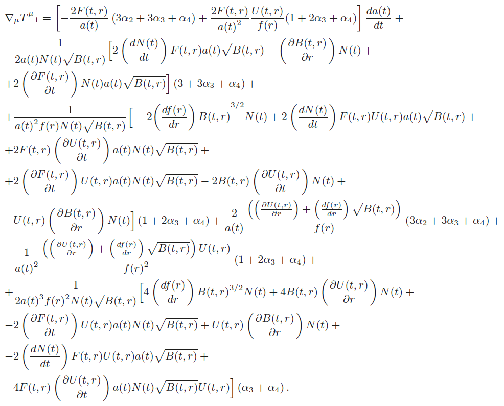
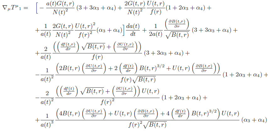
In order to check the viability of such choices for the Stückelberg fields we will consider the conservation of the energy-momentum tensor, ∇μ
In the following sections we present the analysis for the conservation of the energy momentum tensor for several cases, according to the values of α3 and α4 or A(t,r), B(t,r), F(t,r) and G(t,r), depending on which case we are analysing.
3.1. Diagonal Metric
Here we consider that γ, given in (18), is diagonal (G(t,r) = F(r,t) = 0) and the functions A(t,r) and B(t,r) are independent. However, we still have the constraint (16). There are several functions which respect this constraint, but we are interested in cases for which ∇μ
We now analyse some different cases.
3.1.1. A(t,r) = 0, B(t,r) = 4/f(r) 6 and U(t,r) = 1/f(r) 2
The conservation condition (19) gives an expression for T(t,r), which depends on what kind of universe we are dealing with. One can check that T(t,r) is a constant for f(r) = r (flat universe), T(t,r) = ±2coth(r)2 for f (r) = sinh(r) (open universe) and T(t,r) = ±2i cot(r)2 for f(r) = sin(r) (closed universe). Therefore, the equations of motion obtained by varying the action with respect to a(t) and N(t) are, respectively:
and
These are the FLRW equations obtained for the particular choice of A(t,r), B(t,r) and U(t,r). The presence of the anisotropic terms with f(r) means that the solutions are of little interest for cosmology. However if we choose α3 = −1 and α4 = 1, the solutions turn out to be isotropic, with the presence of a cosmological constant-like term, related to the massive graviton mass,
Such solutions are accelerating and could perfectly reproduce the cosmological observations.
3.1.2. U(t,r)=0
In this case we have T(t,r) = constant, which leads to A(t,r) = B(t,r) = 0. The energy-momentum tensor is always conserved and both the fiducial metric and γ are null. Although this seems to be a pathological case, it just reproduces a cosmology with a cosmological constant, represented by the m 2 term, which comes from U(t,r) in the last term of (12). The equations of motion are:
3.1.3. A(t,r) = W(t) 2 , B(t,r) = K(t) 2 and U(t,r) = −K(t)f(r)
When one tries to impose conservation of the energy-momentum tensor it is found that the universe must be open (k = −1), and the relation between W(t) and K(t) is described by
However, the relation (27) together with the conditions for T(t,r) results in a
3.1.4.
With this condition we intend to verify the compatibility of cosmology and massive gravity for Friedmannlike metrics. Such compatibility has been already checked in de Rham et. al. (2014) and states that only an open universe could afford both theories. In some sense this analysis is also present in Volkov (2012a), but the scale factor a(t)2 present in the time component of the physical metric used in Volkov (2012a) does not represents a true FLRW metric. Here we have addressed a similar analysis but we have taken N(t)2 in (14), and after doing calculations the function N(t) is assumed equal to one in order to recover the FLRW background.
Here we present another approach to analyse a solution close to the Friedmann metric. Our choice is to find solutions of T(t,r) and U(t,r) and then try to manipulate them in order to get conservative cases. Besides, we also find results that conserve the energy-momentum tensor like in the previous subsection. By confronting both results we conclude that there is really something special in the theory that excludes solutions for an isotropic and homogeneous fiducial metric.
There are two constraints on the functions T(t,r) and U(t,r) which guarantee diagonality of γ2. By making
After substituting (16) in equation (28) one can find
and
By deriving (29) with respect to t and (30) with respect to r one can combine the results to get:
It is possible to check that T(t,r) has the same solutions of U(t,r) since that function satisfies an equation equivalent to (31). We have chosen U(t,r) = R(r)Z(t) in order to separate the functions of r and t in (31). For this solutions C will stand for the constant of the Fourier method.
When C = 0 the solution is:
where a1, a2, a3 and a4 are constants.
For a positive constant (C > 0) one obtains:
where b1, b2, b3 and b4 are constants.
For a negative constant (C < 0):
with c1, c2, c3, and c4 constants.
By checking equations (32), (33) and (34) it is possible to conclude that both functions U(t,r) and T(t,r) can be modeled in many ways according to the values of the constants. It is worth to pay attention to constant C, which is directly related to the curvature k of the Friedmann metric. That is, after adjusting the constants ai,bi and ci (i=1,2,3,4) to be zero, we can make R(r) mimic f(r).
For instance, when a3 = 0 in (32) we have R(r) = r (a 4 can be absorbed by the temporal part) which is in accord to f(r) = r for k = 0. In equation (33), which corresponds to C > 0, it is possible to obtain f(r) by taking C = 1. This choice recovers f(r) = sinh(r), that represents k = −1. Last but not least, equation (34) corresponds to the closed universe (k = +1) when C = −1 and c4 = 0. For this case R(r) and f(r) are equal to sin(r).
Therefore, one can recover a Friedmann behavior in the r dependent part, which can match a quasi-isotropic metric. Such behavior is desirable once an isotropic and homogeneous metric has already been proved to be compatible only with an open universe.
Some specific cases related to this are:
4.1
For this case we have that u1 is an arbitrary constant. The motion equations are given by
and
4.2
In this case u2 is a constant given by:
The Friedmann equations are:
and
This case is more interesting due its resemblance with the open universe case, which allows compatibility with massivegravity. In this case (Gümrükcuöglu et. al. 2011) the fiducial metricis defined as
and
In the next two sections we analyze massive gravity by considering off-diagonal elements in the function γ given by (18). In Section B we consider that G(t,r) is zero while F(t,r) is non zero. Section D presents the opposite situation (G(t, r) ̸= 0 and F(t, r) = 0). For both cases it is imposed that
3.2. Non-diagonal metric: Case 1
As described previously, this case consists of making F(t,r)
 (42)
(42)
Two different cases are analysed next.
3.2.1. A(t,r) = B(t,r) = 0,F(t,r) = 1/U(t,r) 2 , G(t,r) = 0, α 3 = −2 and α 4 = 3
With this choice there are some restrictions on the functions T(t,r) and U (t,r). By having A(t,r) and B(t,r) null, the only condition is that both are constants or equal. So, it is possible to make U(t,r) equal to a(t)f(r), which would turn this metric closer to the Friedmann one. In any case, the equations of motion are given by
and
Once again, the massive gravity contribution is present as a cosmological constant in the Friedmann equations.
3.2.2. A(t,r) = u 2 N(t) 2 , B(t,r) = u 2 a(t) 2 , U(t,r) = −ua(t)f(r), G(t,r) = 0 and F(t,r) = ua(t)
Here u is a constant to be determined. After some calculation we have the equations of motion:
And
where u is given by:
With a particular choice of α3 = 0 and α4 = −3 we have u = −2 or u = +2/3. Both cases furnish a positive cosmological constant to the mass term, which can also lead to an accelerated expansion.
3.3. Non-diagonal metric: Case 2
Here we follow the same idea of the last subsection, but we have F(t,r) = 0 and G(t,r)
 (48)
(48)
We analyse just one case:
3.3.1. A(t,r)=B(t,r)=U(t,r)=F(t,r)=0 and α 4 =−3(α 3 +1)
This case is dictated by the fact that function (18) has only one non-zero element that is off-diagonal. After squaring it, we see that equation (17) is identically zero. This means that K becomes an identity matrix in the Lagrangian. G(t,r) is an arbitrary function with α4 = −3(α3 + 1) being the only necessary condition for conservation of the energy-momentum tensor. From this we obtain the equations of motion,
and
Both equations (49) and (50) show that massive gravity causes a cosmological constant to appear in the Friedmann equations. For this case it is possible to eliminate the gravitation contribution by making α3= −3.
4. CONCLUSION
In this paper we have obtained new cosmological solutions in the massive gravity theory, constructed by means of to set specific forms for the fiducial metric (15). We found different functions A(t,r), B(t,r), U(t,r) and T(t,r) that guarantee the conservation of the energy-momentum tensor. The equations for the energy momentum tensor conservation were presented in the general form for three different cases, one being diagonal in the fiducial metric and two being non-diagonal. The expressions for the energy-momentum conservation are (19), (20), (42) and (48), the equation for the
Several homogeneous and isotropic solutions that correctly describe an accelerated evolution for the universe were also found, all of them reproducing a cosmological constant term proportional to the graviton mass. From the pairs of equations (23-24), (25-26), (35-36), (38-39), (40-41), (43-44), (45-46) and (49-50) it is easy to see that they can all be reduced to an single equation of the form:
where c(α, u) is a constant function depending on the free parameters α and on the constants u. It is easy to see that the solution to the above equation is:
where the positive solution is a de Sitter type solution, with the property of providing an accelerated expansion to the universe, here sourced by the graviton mass m.
The free parameters α3 and α4 are the contributions coming from the lagrangians counter terms (2) needed to eliminate the Bouware-Deser ghost present in the theory. From a classical point of view, the constants α are as yet unknown, but maybe their values will follow from a perturbative quantum construction of the theory. Although a theoretical approach in order to obtain the values of such constants is not yet available, observational data can provide constraints. (Pereira et. al. 2016).
We have also verified that when the fiducial metric is close to the physical metric the solutions are absent. As already shown in different works, this is a characteristic of the massive gravity theory, which forbids the fiducial metric to be of the same type as the physical one.

