


 nova página do texto(beta)
 Inglês (pdf)
 Artigo em XML
 Referências do artigo
 Enviar este artigo por email
 Citado por SciELO
  Similares em
SciELO
Similares em
SciELO 
 Permalink
1. Introduction
Massive stars are believed to form in dense (n ≈ 103−8 cm−3), cold (T < 30 K), very opaque (τ1001 ≈ 1-6) and massive (M ≈ 8-2000 M⊙) regions, known as pre-stellar cores (Schöier et al. 2002; de Wit et al. 2009; Crimier et al. 2010; Battersby et al. 2014). Chambers et al. (2009) analyzed a significant number of objects having these characteristics and classified them as active cores if they were detected in the mid-infrared (≈ 24 μm), and as quiescent cores if no emission at these wavelengths was measured. These active cores host and form massive stars, whereas inactive cores are excellent candidates for starless massive cores, prior to the onset of the star formation process.
However, unlike low-mass stars (M < 2M⊙), high-mass stars lack a detailed formation scenario. For isolated low mass stars, the shape of the SEDs allows their classification in four evolutionary classes (Shu et al. 1987; Lada 1987; Andre et al. 1993), widely used in the literature. Several factors can be invoked to account for our relatively less detailed knowledge of the formation process/es of high-mass stars (such as: the distances, the relatively small number of massive stars, the amount of energy and winds emitted by these objects, their short evolutionary time, the fact that they are deeply embedded in the cloud material, etc.). One way to help to improve our understanding of the formation scenario of massive stars is to increase the number of young stars with well-determined parameters and to study their environs.
Beltrán et al. (2006) cataloged a large number of massive clumps in the southern hemisphere observed in the infrared (IR) continuum at 1.2 mm. From their list, we selected the source IRAS 08589−4714 (RA, DE[J2000] = 09:00:40.5, -47:25:55) in order to find massive YSOs (young stellar objects) possibly associated with this source and to analyze their evolutionary stage and derive their physical parameters.
IRAS 08589−4714 is located in the giant molecular cloud Vela Molecular Ridge (see zoomed region in the upper panel of Figure 1), which harbors hundreds of low-mass Class I objects and a large number of young massive stars (Lorenzetti et al. 1993). Beltrán et al. (2006) estimated a luminosity of 1.8×10³ L⊙ (compatible with a previous estimate by Wouterloot & Brand 1989) and a mass of 40 M⊙ for this IRAS source. These authors classify the source as an ultracompact HII region (UCHII) since it satisfies the criteria of Wood & Churchwell (1989)2, although no compact radio-continuum source has been detected (Sánchez-Monge et al. 2013). In spite of its high mass, no CH3OH maser emission was found towards this source (Schutte et al. 1993). However, Sánchez Monge et al. (2013) reported water maser emission in the region of the IRAS source.

Fig. 1 Upper panel: Composite image showing the emissions at 250 (red), 160 (green) and 70 μm (blue) from Herschel of the IRAS 08589−4714 region (enclosed by the white rectangle) and including the RCW38 region. Bottom panel: Composite image of the WISE images at 4.6 μm (blue) and 12 μm (green), in combination with the Herschel image at 70 μm (red) of the IRAS 08589−4714 region.
Bronfman et al. (1996) observed the region in the CS(2-1) molecular line. They found that the line had a central velocity VLSR = +4.3 kms−1 and a velocity width at half-maximum ∆V = 2.0 kms-1. In a recent survey, Urquhart et al. (2014) detected emission from the ammonium molecular tracer, NH3, in the (1,1) and (2,2) transitions towards the IRAS source. The central velocity coincides with that of the CS line.
Bearing in mind velocities in the range 4 − 5 km s−1 for IRAS 08589−4714, the circular galactic rotation model by Brand & Blitz (1993) predicts a kinematical distance of 2.0 kpc, with an uncertainty of 0.5 kpc, adopting a velocity dispersion of 2.5 km s−1 for the interstellar molecular gas.
Ghosh et al. (2000) and Molinari et al. (2008) observed this IRAS source in the mid and far infrared and in the sub-millimeter range, and using the IRAS fluxes and those in the J, H , and K bands, measured by Lorenzetti et al. (1993), they constructed and modeled the SED, and found that the IRAS source hasL≈103L⊙,masses between 20-55M⊙, and a B5 spectral type.
The detection of the IRAS 08589−4714 source in the dust continuum, as well as its identification as an UCHII, suggests that it may harbor embedded candidate YSOs. These characteristics make this source an interesting object to investigate the presence of YSOs and their physical properties. In § 2 we present Herschel and WISE data and use the WISE color-color diagram to identify YSOs in the region. In §3 we model the corresponding SEDs to derive infalling envelope parameters, such as: mass, size, density and luminosity. Some of the newly detected young stars show an arc-like structure, in particular at 12 μm, which points to the west, towards the RCW 38 high star-forming region. In § 4 we suggest that RCW 38 may be contributing to the photodissociation of the IRAS source region, shaping the molecular cloud material around the identified young stars. Finally, we present our summary and conclusions in § 5.
2. Infrared sources
2.1. Infrared Data
The source IRAS 08589−4714 was observed with the Herschel space telescope3 (Pilbratt et al. 2010) in the bands of the Photodetector Array Camera and Spectrometer (PACS, 70 and 160 μm; Poglitsch et al. 2010) and of the Spectral and Photometric Imaging Receiver (SPIRE, 250, 350, and 500 μm; Griffin et al. 2010), with nominal FWHM of about, 5'', 12'', 18'',25'', and 36'' in the five bands, respectively. The data were gathered as part of the Herschel Infrared Galactic Plane Survey (Hi-GAL, Molinari et al. 2010), which mapped the Galactic plane in mosaics of ≈ 2.3° x 2.3°, taken in the five bands simultaneously. IRAS 08589−4714 is located in the Hi-GAL field centered at [l, b] = [268.3°, −01.25°]. These mosaics were obtained in the parallel mode, at a scan velocity of 60''/s on 2012 November 13. The raw images were reduced to Level 1, using the HIPE software with standard photometric pipelines. The final maps in Level 2 were processed with the software Scanamorphos, version 24 (Roussel 2013). Finally, we applied appropriate flux correction factors and color corrections to the PACS and SPIRE maps, respectively, according to the corresponding manuals4.
To extract the fluxes in each of the Herschel bands we applied the aperture photometry method, using the HIPE software. We used aperture sizes of 20'' and 25'' in the 70 and 160 μm bands, respectively, and of ≈ 36'' in all three SPIRE bands. The background was estimated over a ring with internal and external radii of ≈ 50'' and 90'', respectively, centered on the peak emission position. The photometric uncertainty assigned to each flux is given by the standard deviation of the measured values after aperture correction. These values are taken at different positions around the central source, without background subtraction, using the same aperture as for the flux measurement of the source (Balog et al. 2013). For IRS 1, 4, 5 and 6 fluxes relative errors are between 10 - 25 %. The remaining sources (IRS 2, 3, and 7) are contaminated by the emission from the environment in which they are immersed and their fluxes for λ > 160 μm have relative errors of ≈ 50 %, preventing us from modeling these sources.
This region was also observed in the bands of the Wide-field Infrared Survey Explorer (WISE) satellite5 (Wright et al. 2010), at W1(3.4 μm), W2(4.6 μm), W3(12 μm), and W4(22 μm), with FWHM of about 6.1'', 6.4'', 6.5'' and 12.0'', respectively. The WISE images and fluxes were obtained from the IRSA (NASA/IPAC Infrared Science Archive6) database.
2.2. Infrared Emission and Identification of YSOs
The bottom panel of Figure 1 is a composite image of the WISE images at 4.6 μm (blue) and 12 μm (green) and the Herschel image at 70 μm (red) of the region IRAS 08589−4714. A vast region dominated by the 70 μm emission is visible on the west. This emission is likely produced by warm dust, while on the east the emission is dominated by colder dust, detected at λ > 100 μm. A transition zone from a hotter to a cooler region is also apparent in this panel (see the highlighted area over the upper panel of Figure 1). A well-defined curved edge that crosses the region from north to south, seen in the W3(12 μm) WISE band (in green) in the bottom panel, is likely produced by the emission of warm dust and polycyclic aromatic hydrocarbons (PAHs; Tielens 2008). For more details on this curved and elongated structure see § 4.
In the bands of the Herschel telescope we detected 7 IR sources (IRS, labeled from 1 to 7 in the bottom panel of Figure 1), four of which (IRS 1, 2, 3, and, 7) were also detected in the bands of the WISE telescope. From the fluxes in these bands, we determined the color indexes of the sources. These four WISE detections are potential Class I or II objects, according to the criteria by Koenig et al. (2012) 7. The left panel of Figure 2 shows the position of these sources in the WISE color-color diagram. The sources without WISE counterparts (IRS 4, 5, and 6) are probably much younger objects (Chambers et al. 2009). IRS 1 and 4 are projected onto two dust clumps (blue contours in Figure 1) identified by Beltrán et al. (2006) at 1.2 mm. Table 1 lists the sources detected in the WISE and Herschel images, with their coordinates and fluxes, and their correlation with the dust clumps detected at 1.2 mm.
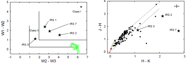
Fig. 2 Left Panel: WISE W1−W2 vs W2−W3 color-color diagram. The dotted lines limit the region where Class I and Class II objects lie according to the Koenig et al. (2012)’s criteria.
Table 1 sources detected towards the IRAS 08589−4714 region using Herschel images and wise counterparts
| Source | α(200.0) | δ(200.0) | F70 | F160 | F250 | F350 | F500 | 1.2a mm |
|---|---|---|---|---|---|---|---|---|
| IRS | (hh:mm:ss) | (°:':'') | (Jy) | (Jy) | (Jy) | (Jy) | (Jy) | (Jy) |
| 1 | 09:00:40.6 | −47:26:01.0 | 236±6 | 343±11 | 201±18 | 88±20 | 25±4 | 1.79±0.17 |
| 2 | 09:00:38.4 | −47:26:48.8 | 6.1±2 | 24±6 | 37±12 | 27±8 | 12±3 | |
| 3 | 09:00:43.1 | −47:25:41.5 | 3.4±1 | 29±8 | 46±18 | 40±16 | 19±9 | |
| 4 | 09:00:48.0 | −47:27:31.4 | 7.5±8 | 44±8 | 53±8 | 29±5 | 11±2 | 0.35±0.03 |
| 5 | 09:00:52.0 | −47:23:47.1 | 11.7±0.7 | 32±4 | 25±3 | 12±1 | 4.9±0.4 | |
| 6 | 09:00:14.5 | −47:27:38.9 | 42±6 | 64±9 | 36±3 | 15±1 | 5.1±0.4 | |
| 7 | 09:00:36.8 | −47:27:17.7 | 5.4±2 | 25±6 | 25±12 | 16±8 | 9±3 | |
| Source | α(200.0) | δ(200.0) | W1(3.4μm) | W2(4.6μm) | W3(12μm) | W4(22μm) | ID WISE | |
| IRS | (hh:mm:ss) | (°:':'') | mag | mag | mag | mag | ||
| 1 | 09:00:40.9 | −47:26:01.1 | 9.46±0.03 | 7.07±0.02 | 4.46±0.02 | 0.22±0.02 | J090040.97−472601.1 | |
| 2 | 09:00:38.6 | −47:26:48.6 | 11.28±0.03 | 9.77±0.03 | 5.61±0.03 | 2.80±0.04 | J090038.59−472648.5 | |
| 3 | 09:00:43.1 | −47:25:39.6 | 9.35±0.02 | 8.24±0.02 | 6.63±0.03 | 3.04±0.03 | J090043.08−472539.5 | |
| 7 | 09:00:37.1 | −47:27:17.6 | 10.13±0.03 | 8.21±0.02 | 5.10±0.03 | 2.80±0.06 | J090037.06−472718.4 | |
Green open squares on the left panel of Figure 2 correspond to faint WISE sources that lie in the region of the WISE color-color diagram contaminated by PAH emission, according to Koenig et al. (2012) 8. PAH emission has prominent lines in the WISE band W1 and W3, producing color excesses (Wright et al. 2010). These sources are listed in Table 2. Interestingly, these objects are spatially located around the arc-shaped structures near IRS 1, 5 and 6. Figure 3 shows the bottom panel of Figure 1 (4.6 μm in blue, 12 μm in green, and 70 μm in red), indicating with red triangles the positions of these faint WISE sources. None of these sources has been detected in the Herschel bands, with the exception of those coincident with IRS 5 and 6. All sources in Table 2 are potential or candidate YSOs that require deeper observations to confirm their nature and evolutionary status.
Table 2 Wise sources detected towards IRAS 08589−4714 likely contaminated with PAH emission
| ID | α(200.0) | δ(200.0) | W1(3.4μm) | W2(4.6μm) | W3(12μm) | W4(22μm) | ID WISE |
| (hh:mm:ss) | (°:':'') | mag | mag | mag | mag | ||
| WISE1 | 9:00:12.9 | -47:27:22.5 | 11.34±0.04 | 10.76±0.03 | 5.22±0.02 | 3.34±0.05 | J090012.96−472722.5 |
| WISE2 | 9:00:14.1 | -47:27:48.0 | 11.19±0.03 | 10.96±0.06 | 5.03±0.02 | 3.20±0.07 | J090014.11−472748.0 |
| WISE3 | 9:00:45.1 | -47:26:59.9 | 12.92±0.08 | 12.53±0.08 | 6.44±0.05 | 3.25±0.03 | J090045.14−472659.8 |
| WISE4 | 9:00:57.2 | -47:29:03.7 | 12.72±0.06 | 12.59±0.09 | 6.55±0.05 | 4.64±0.06 | J090057.28−472903.7 |
| WISE5 | 9:00:32.7 | -47:26:58.4 | 13.09±0.08 | 13.03±0.07 | 7.21±0.11 | 4.80±0.06 | J090032.72−472658.4 |
| WISE6 | 9:00:46.5 | -47:27:47.5 | 12.25±0.05 | 12.29±0.07 | 6.25±0.02 | 4.19±0.04 | J090046.52−472747.5 |
| WISE7 | 9:00:55.6 | -47:28:16.3 | 12.79±0.12 | 12.21±0.11 | 6.78±0.15 | 4.29±0.14 | J090055.55−472816.2 |
| WISE8a | 9:01:01.0 | -47:29:28.5 | 12.63±0.04 | 12.59±0.06 | 6.95±0.07 | 4.24±0.05 | J090101.00−472928.4 |
| WISE9a | 9:00:55.8 | -47:27:03.6 | 13.36±0.13 | 12.99±0.15 | 7.63±0.18 | 5.87±0.47 | J090055.83−472703.5 |
| WISE10 | 9:01:02.0 | -47:27:17.8 | 13.05±0.09 | 12.58±0.09 | 6.71±0.06 | 4.42±0.07 | J090101.97−472717.8 |
| WISE11 | 9:00:37.2 | -47:25:43.9 | 11.76±0.05 | 11.54±0.04 | 5.58±0.03 | 3.67±0.06 | J090037.21−472543.9 |
| WISE12a | 9:00:55.2 | -47:29:33.6 | 12.45±0.03 | 12.70±0.05 | 6.58±0.02 | 4.85±0.05 | J090055.21−472933.5 |
| WISE13 | 9:00:40.7 | -47:24:00.8 | 12.55±0.04 | 12.22±0.05 | 6.45±0.03 | 4.69±0.12 | J090040.76−472400.7 |
| WISE14 | 9:00:51.8 | -47:23:55.4 | 12.06±0.03 | 11.92±0.04 | 6.00±0.02 | 3.64±0.04 | J090051.82−472355.3 |
| WISE15 | 9:00:52.0 | -47:23:30.6 | 12.73±0.05 | 12.25±0.06 | 6.58±0.04 | 4.22±0.07 | J090052.00−472330.6 |
aSource with 2MASS counterpart.
The right panel of Figure 2 shows the 2MASS near-IR color-color J − H vs H − K diagram of the IRAS 08589−4714 region. IRS 2, 3 and 7 have near IR color excesses. Another three sources with near IR color excess lie in the direction towards IRS 1. All these 2MASS sources, located to the right of the reddening band, are listed in Table 3. The 2MASS sources coincident with IRS 5 and 6 do not have color excess in these bands (they are not included in Table 3). These sources are marked in Figure 3 with red squares. Color excesses in the near and middle IR could be associated with warmer dust in the inner part of the envelope, which could be due to a circumstellar disk (Sicilia-Aguilar et al. 2006). This would confirm that these sources are young.
Table 3 2MASS sources detected towards IRAS 08589−4714 with near-IR excesses
| ID | α(200.0) | δ(200.0) | J(1.2 μm) | H (1.6 μm) | Ks(2.2 μm) | ID 2MASS |
| (hh:mm:ss) | (°:':'') | mag | mag | mag | ||
| 2MASS 1a | 9:00:41.4 | -47:26:05.0 | 16.38±0.13 | 13.59±0.06 | 11.75±0.04 | 09004142−4726050 |
| 2MASS 2a | 9:00:42.0 | -47:26:00.3 | 13.8±0.2 | 12.7±0.2 | 11.43±0.05 | 09004201−4726002 |
| 2MASS 3a | 9:00:42.3 | -47:25:59.3 | 13.61±0.04 | 12.94±0.05 | 11.5±0.1 | 09004229−4725593 |
| 2MASS 4 (IRS 3) | 9:00:43.1 | -47:25:39.5 | 13.82±0.03 | 12.13±0.03 | 11.00±0.03 | 09004309−4725394 |
| 2MASS 5 (IRS 2) | 9:00:38.6 | -47:26:49.0 | 18.5±0.2 | 15.64±0.13 | 13.51±0.07 | 09003861−4726489 |
| 2MASS 6 (IRS 7) | 9:00:37.1 | -47:27:18.4 | 17.4±0.2 | 15.77±0.15 | 12.99±0.03 | 09003706−4727184 |
| 2MASS 7 | 9:00:42.9 | -47:25:52.3 | 16.8±0.2 | 15.22±0.11 | 13.98±0.08 | 09004292−4725522 |
aSource in the direction towards IRS 1.
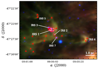
Fig. 3 Composite image of the WISE images at 4.6 μm (blue) and 12 μm (green), in combination with the Herschel image at 70 μm (red) of the IRAS 08589−4714 region. Red triangles show the positions of faint WISE sources listed in Table 2. Red squares correspond to sources with near-IR excesses listed in Table 3. The color figure can be viewed online.
3. Analysis of the infrared sources
3.1. The Spectral Energy Distributions
In this Section, we analyze the evolutionary status of some of the sources identified in the Herschel images (see § 2.2) by means of their SEDs. To construct the SEDs we use the fluxes in the Herschel bands at 70, 160, 250, 350, and 500 μm. Since protostars lie embedded in dense and opaque material we can derive the main characteristics of the envelopes surrounding the central objects. Fluxes for λ < 20μm are excluded from the modeling of the whole set of sources since the code used (DUSTY, see § 3.3) underestimates the emission at these wavelengths. This is commonly observed in spherically symmetric models that do not include cavities or inhomogeneities in the envelope to allow radiation at these wavelengths to escape.
In the case of IRS 1, we model the SED and the 70 μm radial intensity profile (see § 3.2) simultaneously, while for IRS 4, 5, and 6 we model the corresponding SEDs only, since they are too faint to obtain reliable profiles at 70 μm. In the SED corresponding to IRS 1 we include the 1.2 mm flux from Beltrán et al. (2006) and the flux at 22 μm from WISE, while in the case of the SED for IRS 4 we only include the flux at 1.2 mm. This source does not have a mid-IR counterpart. The SED of IRS 1 is shown in the left panel of Figure 4, and those of IRS 4, 5, and 6, in Figure 5.
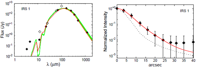
Fig. 4 SED (left panel) and intensity profile at 70 μm (right panel) of IRS 1. The filled diamonds correspond to the fluxes from the Herschel and WISE telescopes.
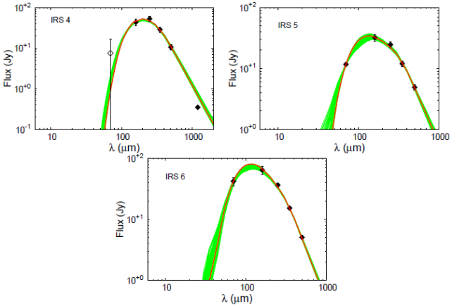
Fig. 5 SEDs of IRS 4 (left top panel), 5 (right top panel), and 6 (left bottom panel). The filled diamonds belong to the five Herschel bands. The empty diamond in the SED for IRS 4 is an upper limit to the 70 μm flux. The error bars are included. The relative errors in the fluxes are between 10 and 25%.
3.2. The 70 μm Intensity Profile for IRS 1
The average azimuthal intensity profile is commonly employed to compare modeled and observed images. This is used to complement the analysis of SEDs, as it allows to reduce the number of free parameters, and thus minimizes the degeneration of the solutions (Crimier et al. 2010). We present the modeling of the intensity profile at 70 μm corresponding to IRS 1.
Since the PSF (point spread function) at 70 μm is rather elongated (due to the scan speed, which for 60''/s gives a PSF of 5.83'' x 12.12'', Poglitsch et al. 2010), to determine the radial intensity profile several one-dimension radial profiles are obtained in different directions from the center of the source. In the case of IRS 1 (see Figure 4), we use only the hemisphere in the opposite direction to the apex of the curved structure seen in Figure 1 to avoid contamination from the surrounding diffuse and extended emissions. The uncertainty in the profile is given by the noise in the image and the non-circularity of the beam of the source. The latter effect is taken into account by the standard deviation of the average azimuthal flux. The profile is normalized by its maximum value.
3.3. The Fitting Method
The SEDs of the four sources, as well as the 70 μm intensity profile of IRS 1, were modeled with the DUSTY9 code of Ivezic & Elitzur (1997). The code solves the radiative transfer in one dimension for a dusty shell that surrounds a central source, which emits as a black body and whose radiation is absorbed, scattered and re-emitted by the dust in the envelope. This envelope has a density profile that follows a power law (n ∝ r−p), and it is parameterized by the relative size given by Y = rext /rin, where rext and rin are the external and internal radii of the shell. The temperature of the central source (Tstar) and the temperature at the internal radius of the envelope (Tin) are fixed, with values of 15000 and 300 K, respectively. The results are rather insensitive to the values of Tstar.
We tested the DUSTY SEDs for Tstar between 5000 and 50000K, and no distinguishable differences in the results were found. On the other hand, the inner radius was relatively unconstrained by current data resolution (5'' corresponds to ≈ 10 000 AU at 2 kpc), as is Tin. As a matter of fact, Tin determines the radius at which the code starts the calculations. Several SEDs models of massive stars, as well as mid-infrared spectra rule out inner radius temperatures consistent with dust sublimation temperatures (≈ 1500 K). Radiation pressure, stellar winds and/or shocks are usually invoked to produce a large cavity depleted of dust and to limit the amount of short wavelength emission (Churchwell et al. 1990; Faison et al. 1998; Hatchell et al. 2000). For Tin we fixed a value in a manner similar to previous work, adopting an inner radius larger than would be expected from dust sublimation (Hatchell et al. 2000; Jørgensen et al. 2002; Crimier et al. 2009, 2010; Vehoff et al. 2010; Hirsch et al. 2012). Finally, for very young sources it is usual to assume that the envelope is composed of particles surrounded by a thin layer of ice. For this reason, we adopted the opacity corresponding to a density of 106 cm−3 from Ossenkopf & Henning (1994).
The DUSTY model needs to be scaled to the distance and the bolometric luminosity (Lbol) of the central source so as to compare the models and observed data. The bolometric luminosity is, however, an output parameter, since it is calculated by integrating the modeled SED. Consequently, the luminosity is re-evaluated as input parameter iteratively until the difference between the models and observations is minimized. We adopted a distance of 2.0 kpc (see § 1), assuming that all the sources belong to the IRAS 08589−4714 region.
On the other hand, the intensity profiles modeled by DUSTY show an intense and very narrow central component (width < 1''). This component is the stellar radiation attenuated by a dusty envelope, whose width is proportional to the stellar radius (Ivezić & Elitzur 1996). Given that the pixel size at 70 μm is 3′′.2, we re-binned the model profile using a slightly larger bin of 4′′. Finally, this profile is convolved with the instrumental profile at 70 μm, taken as the average intensity profile of PACS calibrated sources, such as α Tau, the Red Rectangle, IK Tau and the Vesta asteroid (Lutz 2012). The first two sources are used to model the core and the last two the extended wings of the profile (Aniano et al. 2011).
To systematically compare the models with the observations we built a grid of 127 100 DUSTY models. The grid was constructed for 31 values of the power index (p) in the density profile, ranging from 0.0 to 3.0 in steps of 0.1, 82 values of the envelope relative size (Y) in the range 100-910 with steps of 10, and 50 values of the optical depth (τ100), from 0.1 to 5.0, in steps of 0.1. The space of the parameters explored is similar to that used by Crimier et al. (2010), restricted to a more limited range of each parameter but including typical values for young stellar objects. Table 4 summarizes the ranges of the free parameters. The best fit is obtained by means of the goodness-of-fit criterion. We employed the weighted least squares method to fit the SED. The weights are inversely proportional to the square of the errors assigned to each observed data point.
Table 4 Range explored with dusty for different parametersParameter
| Parameter | Range | Step |
| p | 0.0-3.0 | 0.1 |
| Y | 100-910 | 10 |
| τ100 | 0.1-5.0 | 0.1 |
| Tstar | 15000 K | - |
| Tin | 300 K | - |
In the case of IRS 1, to find a model that fits both the SED and the intensity profile simultaneously we followed the procedure used by Crimier et al. (2010). We first fixed the value of the opacity (τ100) and, by fitting the intensity profile, we obtained an initial value for the power law index (p) and for the envelope relative size (Y). Then we recalculated the value of τ100 by fitting the SED, using the values of p and Y derived in the previous step. We adopted the new value of τ100 in the next iteration, and the process was repeated. Convergence was achieved in a few steps. This procedure considers the fact that the intensity profile is strongly dependent on the size of the envelope and the density distribution, whereas the SED depends mainly on the column density, that, in turn, depends on the opacity (Crimier et al. 2010).
3.4. Derived Parameters
The solid red line in Figures 4 and 5 shows the best DUSTY models for IRS 1, 4, 5, and 6. With green continuous line we show all DUSTY models comprised within the error bars of the fluxes (20 in the case of IRS 1 and 200 for IRS 4, 5 and 6). Table 5 summarizes the parameters that best reproduce the data: the luminosity L, the opacity τ100, the power law index p, and the relative size of the envelope Y. We include in this table the physical parameters of the envelope: the inner rin and external, rext radii, the temperature of the dust at rext, Tdust, and the mass, Menv and density in the inner part of the envelope n(rin).
Table 5 Best modeled parameters
| Input model parameters | |||||
| IRS | L | τ100 | p | Y | |
| (L⊙) | |||||
| 1 | 1.9×10³ | 0.2 | 0.0 | 250 | |
| 4 | 1.2×10² | 4.8 | 0.4 | 130 | |
| 5 | 1.2×10² | 3.9 | 1.7 | 410 | |
| 6 | 3.0×10² | 5.0 | 2.1 | 110 | |
| Derived physical parameters | |||||
| IRS | rin | rext | Tdust | Menv | n(rin) |
| (AU) | (pc) | (K) | (M⊙) | (cm-3) | |
| 1 | 112 | 0.14 | 18 | 86 | 3×10⁵ |
| 4 | 36 | 0.02 | 16 | 42 | 2×10⁷ |
| 5 | 66 | 0.13 | 10 | 38 | 1×10⁷ |
| 6 | 129 | 0.07 | 11 | 11 | 7×10⁶ |
Since the DUSTY code does not provide error determinations for the modeled parameters, Table 6 lists average values and standard deviations corresponding to all DUSTY models (calculated for the same luminosity) that fall within the error bars of the fluxes (green lines in Figs. 4 and 5). Best model parameters listed in Table 5 are not always within the standard deviations given in Table 6. However, they are not significantly different from the average values. In the case of IRS 1, p and Y are derived by modeling simultaneously the SED and the 70 μm intensity profile. For this reason, the differences between the values listed in Table 5 and 6 are larger.
Table 6 Average modeled parameters
| Average input parameters | |||||
| IRS | τ100 | p | Y | ||
| 1 | 0.3±0.0* | 0.8±0.1 | 330±53 | ||
| 4 | 3.3±1.0 | 0.4±0.3 | 214±56 | ||
| 5 | 3.0±1.5 | 1.4±0.4 | 447±176 | ||
| 6 | 2.7±1.5 | 1.5±0.6 | 170±62 | ||
| Average derived physical parameters | |||||
| IRS | rin | rext | Tdust | Menv | n(rin) |
| (AU) | (pc) | (K) | (M⊙) | (cm-3) | |
| 1 | 129±2 | 0.21±0.03 | 16±1 | 124±33 | (4.00±0.02)×105 |
| 4 | 35±5 | 0.04±0.01 | 14±2 | 60±12 | (1.6±0.4) ×107 |
| 5 | 56±16 | 0.13±0.08 | 11±2 | 38±14 | (8.4±2.5) ×106 |
| 6 | 89±29 | 0.08±0.05 | 15±3 | 15±3 | (4.9±1.3) ×106 |
* All models that fall within the fluxes error bars have the same τ100 value.
For the SED of IRS 1, the fluxes at 3.4, 4.6, and 12 μm are not well fitted by the model, as we have mentioned before. These fluxes are likely contaminated by shocks and PAH emission features detected in these WISE bands (Wright et al. 2010). Moreover, Saldaño et al. (2016) detected an outflow associated with IRS 1, which likely produces a cavity in the envelope. Dust in the walls of the cavity is heated by UV and optical radiation coming from the stellar embryo/s, re-irradiating in the IR (see, for example, Bruderer et al. 2009; Zhang et al. 2013). Thus mid-IR fluxes are considered to be upper limits. In addition, the observed intensity profile is well fitted by the modeled profile out to 20'', but not beyond.
The density profile for the envelope of IRS 1 derived with the DUSTY code is constant, and consistent with the supposition introduced by Ghosh et al. (2000) in their model of the SED of this source. In addition, the other parameters determined by these authors (M = 55 M⊙, Rmax = 0.2 pc, L = 2.4 ×10³ L⊙) are similar or of the same order as the parameters obtained through DUSTY. However, we derived an opacity for the envelope four times larger than the value obtained by Ghosh et al. (2000). The difference is probably due to the fact that these authors used silicate and graphite dust grains without a layer of ice on the surface, producing less attenuation to the radiation. The inclusion of a layer of ice gives a more realistic model (Ossenkopf & Henning 1994).
3.5. Virial Mass
Assuming that: (1) the parent cloud is similar to that one used in the DUSTY code; (2) the source is in hydrostatic equilibrium; and (3) the volume density of the gas decays as a power law (ρ ∝ r−p), we estimate the envelope mass using the following expression for the virial theorem:
where G is the gravitational constant and σ is the one-dimensional velocity dispersion averaged over the entire system. The k factor is approximately equal to 1 for Y ≫1 and p<2.5. Using the parameters calculated by the DUSTY code, such as p and r
ext
, and
4. Probable scenario for the origin of the arc-like structures
In Figure 6 we show large scale WISE and Herschel images of the region of the IRAS 08589−4714 source with the aim of explaining the arc-like structures detected mainly at 12 μm. We superimpose contour lines of the emissions at 12 μm from WISE (green lines) and at 1.2 mm (blue lines) from Beltrán et al. (2006). The seven sources identified and labeled in Figure 1 are also marked in the 4.6 μm image.

Fig. 6 WISE 4.6 μm and Herschel 70, 160 and 500 μm images of the IRAS 08589−4714 region. Blue contours correspond to the 1.2 mm emission (Beltrán et al. 2006) and those in green to the WISE 12 μm emission. The sources labeled IRS 1 to 7 correspond to those in Table 1. The color figure can be viewed online.
At 12 μm we can see three arc-like structures pointing to the west. The more extended structure borders the western rim of IRS 1, and the two smaller ones coincide with IRS 5 and 6. Saldaño et al. (2016) observed 12CO(3−2), 13CO(3−2), C18 O(3−2), HCO+ (3−2), and HCN(3−2) molecular lines in a region of 150′′ × 150′′, centered on the IRAS source with the APEX telescope. These data covered IRS 1 and 3 positions. The molecular emissions of 12CO and 13CO to the west of IRS 1 are lower (Tmb < 2K) than in the east side (Tmb > 10K). In addition, the integrated emission of 13CO shows a very steep intensity gradient to the west, suggesting that the material linked to IRS 1 is being compressed. Finally, in Figure 6 we can see that the emission at 12 μm borders the western rim of the cold dust emission, as it is better seen in the 160 and 500 μm images. The WISE filter at 12 μm (with a bandwidth ≈ 9 μm) includes strong spectral lines of neutral and ionized PAH (Tielens 2008), typical of photodissociation regions (PDRs). The comparison of the emission at 12 μm, likely from ionized PAHs, and at 1.2 mm, from cold dust, suggests the existence of hot sources located to the west, which are creating a PDR bordering the molecular gas.
We have used the 70 and 160 μm Herschel images to obtain a dust temperature map at the highest angular resolution possible in a relatively small area. In addition, these bands are good tracers of warm dust, a likely scenario for IRAS 08589−4714 since not only it is exposed to an intense external radiation field but it also contains embedded YSO candidates. The map was constructed as the inverse function of the ratio of Herschel 70 and 160 μm maps, i.e., Tc = f (T)−1 . Assuming a dust emissivity following a power law κν ∝ νβ, β being the spectral index of the thermal dust emission, in the optically thin thermal dust emission regime f (T) has the form:
where B(70, T) and B(160, T) are the blackbody Planck function for a temperature T at wavelengths 70 μm and 160 μm, respectively. The pixel-to-pixel temperature was calculated assuming a typical value β = 2.
In Figure 7 we show the color-temperature map obtained using the method explained above. For temperatures in the range ≈ 20-40 K, the uncertainty of the derived dust temperatures using this method was estimated to be about ≈ 10-25 %. Also, Figure 1 shows that the interstellar dust to the west of the sources appears warmer than to the east because of the presence of emission at smaller wavelengths. Figure 7 suggests the existence of a gradient in the dust temperature, with the lower values towards the east. Note in particular the regions to the east of IRS 5 and 6, where dust appears to be shielded from UV photons. We caution that ≈ 40% of the area shown in Figure 7 has temperatures < 20 K, a range where, as mentioned, uncertainties may be large. However, any overestimation makes the gradient less steep. In other words, real temperatures below 20 K would be even lower than shown in this figure and the gradient steeper. Thus, the gradient from west to east exists, in spite of the uncertainties in T. However ≈ 60% of the area shown in Figure 7 is dominated by a relatively warmer component that prevails in the emission at 70 μm towards the west, which likely indicates the influence of RCW 38.

Fig. 7 Dust temperature map (in color scale) derived from Herschel emission at 70 and 160 μm. The colortemperature scale (in K) is on the right. The white cross indicates the IRAS source position. The arrows mark the positions of IRS 5 and 6, as references.
About 16'.7 to the west of IRAS 08589−4714 lies the high mass star-forming region RCW 38 (upper panel of Figure 1). This HII region is excited by an O5.5 binary star (RCW38 IRS 2; DeRose et al. 2009). In addition, Winston et al. (2011) report the detection of a dozen O-type stars and several candidate OB stars associated with RCW38. Many of these sources are ionizing the interstellar medium, generating HII regions located in the surrounding area (Kuchar & Clark 1997; Yamaguchi et al. 1999; Paladini et al. 2003; Brown et al. 2014; Anderson et al. 2014). Figure 8 indicates the location of these HII regions. Moreover, the center of RCW38 shows strong X-ray activity that may be produced by the formation of massive stars. There are, at least, 50 sources emitting at these wavelengths (Kuhn et al. 2013; Broos et al. 2013). RCW 38 is located at a distance of 1.7 kpc (Stead & Hoare 2009), similar, within errors, to the distance of IRAS 08589−4714 (2.0 ± 0.5 kpc). The center of the RCW 38 lies ≈ 10 pc away from the center of the IRAS 08589−4714 region.
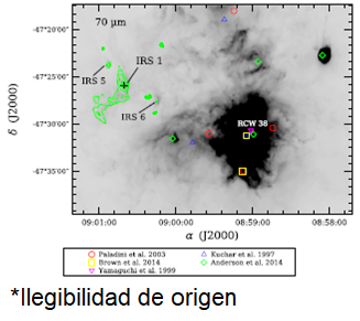
Fig. 8 70 μm Herschel images of the WCR 38 region showing the locations of different HII regions. References are included at the bottom of the figures. The cross shows the position of the IRAS 08589−4714 source, on top of which 70 μm contours are superimposed. The color figure can be viewed online.
Kaneda et al. (2013) carried out a large-scale mapping of RCW38 in the [CII] and PAH emissions. They found that the [CII] (158 μm) emission extends about 10′ (about 5 pc) away from the center of RCW38, in particular in the north and east directions. Sources IRS 1, 2, 7 and 6 lie about 2.5′ or about 1.5 pc away from the most external [CII] contour. It is noteworthy that [CII] is considered one of the main cooling agents of low-density photodissociation regions with PAHs emissions (see, for example, Hollenbach & Tielens 1999; Goicoechea et al. 2003) and, therefore, a good tracer of them. In addition, [CII] emission strongly correlates with PAHs emissions. Consequently, it is likely that massive stars in RCW38 are photodissociating the molecular gas producing the PDR and heating the interstellar dust to the west of IRAS 08589−4714.
5. Summary and conclusions
We used WISE 3.4, 4.6, 12 and 22 μm and Herschel 70, 160, 250, 350 and 500 μm fluxes to analyze 7 sources identified in the IRAS 08589−4714 region. Four of these sources (called IRS 1, 2, 3 and 7) have WISE colors of Class I and II objects, according to the criteria of Koenig et al. (2012). The other three (IRS 4, 5 and 6) have no midinfrared counterparts and are likely to be younger objects (Chambers et al. 2009). We modeled the SEDs in the range 20-1200 μm for the four brightest sources in these wavelengths (IRS 1, 4, 5 and 6), deriving physical parameters for the associated envelopes, such as envelope masses, sizes, densities, and luminosities. These parameters range from 16 to 68 M⊙, 0.06 - 0.12 pc, 9.6×10⁴ - 9.2×106 cm−3, and 0.12 - 2.6×10³ L⊙, suggesting that these sources are very young, massive and luminous objects at early stages of the formation process.
We constructed the color-color diagrams in the bands of WISE and 2MASS to identify potential young objects in the region. Those identified in the bands of WISE are contaminated by the emission of PAHs, except four sources (IRS 1, 2, 3 and 7). These faint candidates require more sensitive observations to confirm their nature and evolutionary status.
In the WISE 12 μm band, we identified an arclike structure linked to IRS 1, pointing to the west, and another two smaller structures coinciding with the positions of two infrared sources (IRS 5 and 6) lying in the region, with similar shapes and pointing in the same direction. The massive star-forming region RWC 38, harboring a dozen of O-type stars, is located ≈ 16.'7 from these sources in the west direction and roughly at the same distance. The ultraviolet photon flux from the exciting stars of RCW 38 is probably photo dissociating the material in the IRAS 08589−4714 region and creating a photo dissociated region.

