


 nueva página del texto (beta)
 Inglés (pdf)
 Artículo en XML
 Referencias del artículo
 Enviar artículo por email
 Citado por SciELO
  Similares en
SciELO
Similares en
SciELO 
 Permalink
1. Introduction
Very little has been done on BO Lyn since its discovery by Kinman et al. (1994) (as reported by Kazarovets & Samus, 1997, star 73243 in their Table 1). Kinman (1998) analyzed the star and assigned to it a period of 0.0933584 days and a V -magnitude range of 11.85-12.05 with a slightly variable light curve. He further stated that “the location, space motion, and other properties of this star indicate that it is a higher amplitude δ Scuti star (or ‘dwarf Cepheid’) that is a member of the old disk population”. The most recent study was done by Hintz et al. (2005) who examined the star both photometrically and spectroscopically and proposed that the period is decreasing at a constant rate.
Table 1 Log of observing seasons.
| Date | Telescope | Npoints | ΔT (d) | ΔV | Observers* |
|---|---|---|---|---|---|
| 16/01/1112 | 84 cm | 37 | 0.079 | 0.054 | aas, jg |
| 16/01/1314 | 84 cm | 41 | 0.086 | 0.054 | aas, jg |
| 16/01/2122 | 14 inch | 297 | 0.228 | 0.020 | ESAOBELA16 |
| 16/01/2324 | 14 inch | 266 | 0.123 | 0.018 | ESAOBELA16 |
| 16/01/2425 | 14 inch | 356 | 0.165 | 0.020 | ESAOBELA16 |
| 16/02/0607 | 10 inch | 469 | 0.227 | 0.031 | jg, ap |
*aas, A.A. Soni; jg, J. Guillén; ap, A. Pani; ESAOBELA16: A. Rodríguez; V. Valera; A. Escobar; M. Agudelo; A. Osorto; J. Aguilar; R. Arango; C. Rojas; J. Gomez; J. Osorio; M. Chacon.
2. Observations
This star was observed at both the Observatorio Astronómico Nacional of San Pedro Mártir, México with the 0.84 m telescope and a uvby−β spectrophotometer and at Tonantzintla, México with 14-inch and 10-inch telescopes provided with SBIG ST 8300 and ST1001 CCD cameras, respectively. The log of the observations is given in Table 1. Column 1 reports the date (year month day), Column 2 the tele-scope and implicitly, the observatory; Columns 3 and 4 the number of points and the time span of the observations; Column 5 the uncertainty in each night; it should be kept in mind that in the first two rows we present the uncertainty in the absolute transformation to the standard system and in the remaining rows, the error of differential magnitudes; finally, the last column lists the observers.
2.1. Data Acquisition and Reduction at Tonantzintla
During all the observational nights the following procedure was utilized. Sequence strings were obtained in the V filter with an integration time of 30 sec. There were 551,111 counts for BO Lyn, 1,555,128 for the comparison star C1 and 2,774,289 counts for the check star C2, enough counts to secure high accuracy. The error in each measurement is, of course, a function of both the spectral type and the brightness of each star but they were observed long enough to secure sufficient photons to get a good S/N ratio and an observational error of 0.001 mag in all cases. The reduction work was done with AstroImageJ (Collins, 2012). This software is relatively easy to use and has the advantage that it is free and works satisfactorily on the most common computing platforms.
For the CCD photometry of BO Lyn (08:43:01.224, +40:59:51.79) two reference stars were utilized. A bright star TYC 2985-290-1 identified in the present paper as C1 (08:42:39.883, +40:59:48.30, V = 10.91, SpT= N/A) was used as comparison star, and a brighter star, BD +41 1869, identified as C2 (08:42:33.428, +41:05:59.97, V = 10.30, SpT=F8) as a check star to obtain the light curves in a differential photometry mode. The reason for using the less bright star C1 as a comparison object instead of C2 is that, during the observation, C2 was out of the observed field near the time of maximum due to the rotation of the telescope caused by the alt-azimuthal mounting. The results were obtained from the difference Vvariable - Vcomparison and the scatter calculated from the difference Vcomparison − Vcheck. Each of these times of maxima has an accuracy of 3 × 10⁻⁴ day. Figure 1 presents the light curves of BO Lyn.

3. O-C analysis
To investigate the secular behavior of the period of BO Lyn we studied the literature related to it. Besides Kinman (1998) only two groups of researchers have observed BO Lyn: Klingenberg et al. (2006) with few observations and, previously, Hintz et al. (2005) who performed studies of the O-C behavior of this star. A summary of their findings is presented in Table 2. In Column 1 the author is presented, Column 2, 3 and 4 the ephemerides determined by each author; T0, P and β respectively. Columns 5 and 6 list the mean value of the (O-C) for all the times of maximum light and the standard deviation, respectively. Hubscher et al. (2013) published only one time of maximum light. All are presented schematically in Figure 2.
Table 2 BO Lyn ephemerides equations.
| Author | T 0 | P | β | (O-C)mean | (O-C)std dev |
|---|---|---|---|---|---|
| Kinman (1998) | 2438788.0355 | 0.0933584 | −0.021 | 0.028 | |
| Hintz et al. (2005) linear | 2447933.8183 | 0.09335724 | −0.007 | 0.014 | |
| Hintz et al. (2005) parabolic | 2447933.7988 | 0.09335800 | −7.2(1.0) ×10−12 | −0.001 | 0.009 |
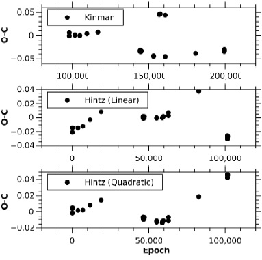
Table 3 lists the observed times of maximum light of BO Lyn and includes the new observations. In this table, Column 1 reports the time of maximum light (in HJD), Column 2, the source and Column 3 the epoch with the ephemerides parameters determined in this paper.
Table 3 Times of máxima of BO Lyn.
| Time of Maximum | Reference | Epoch |
|---|---|---|
| 2447933.7964 | Hintz-Kinman | 0 |
| 2447938.7478 | Hintz-Kinman | 53 |
| 2448274.9308 | Kinman | 3654 |
| 2448577.9691 | Hintz-Kinman | 6900 |
| 2449010.7845 | Kinman | 11536 |
| 2449685.9520 | Kinman | 18768 |
| 2452252.8044 | Hintz | 46263 |
| 2452252.8993 | Hintz | 46264 |
| 2452264.7545 | Hintz | 46391 |
| 2452264.8459 | Hintz | 46392 |
| 2452266.7141 | Hintz | 46412 |
| 2452266.8091 | Hintz | 46413 |
| 2452288.6538 | Hintz | 46647 |
| 2452288.7455 | Hintz | 46648 |
| 2452288.8399 | Hintz | 46649 |
| 2452310.6849 | Hintz | 46883 |
| 2452331.7861 | Hintz | 47109 |
| 2453075.7484 | Hintz | 55078 |
| 2453075.8406 | Hintz | 55079 |
| 2453083.7767 | Hintz | 55164 |
| 2453427.7978 | Hintz | 58849 |
| 2453429.7592 | Hintz | 58870 |
| 2453487.7356 | Hintz | 59491 |
| 2453795.5356 | Klingenberg | 62788 |
| 2453795.6334 | Klingenberg | 62789 |
| 2455654.4061 | Hubscher | 82699 |
| 2457409.7380 | Esaobela16 | 101501 |
| 2457409.8276 | Esaobela16 | 101502 |
| 2457409.9249 | Esaobela16 | 101503 |
| 2457411.7932 | Esaobela16 | 101523 |
| 2457412.7228 | Esaobela16 | 101533 |
| 2457412.8180 | Esaobela16 | 101534 |
| 2457425.7953 | jg, aas | 101673 |
| 2457425.8890 | jg, aas | 101674 |
Since the study of Hintz et al. (2005), more observations have been carried out, some of them recently, and they are presented in this paper in Table 3. We tested the old proposed ephemerides equations with the complete set of times of maximum light which is constituted of a set of only 34 times of maximum light including those observed in 2016 (Figure 2). At the time of the Hintz et al. (2005) study, the time basis was only 5554 days or 15 years. In 2016 the time basis has been extended to 9492 days or 26 years, almost double that used for the calculations of Hintz et al (2005).
4. Period determination
To determine the period behavior of BO Lyn we followed three methods.
4.1. Period04
In this method all detailed photometry was used: Kinman (1998) which is presented in apparent magnitudes, and that of the present paper which includes that observed at the Tonantzintla and San Pedro Martir Observartories, Mexico and, as has been explained, consisted of two samples: absolute photometry in San Pedro Martir for two nights and differential photometry in Tonantzintla for four nights. Because of the amplitude difference between the instrumental and the apparent magnitudes and for a consistent analysis, all the light curves were normalized subtracting the average of each night from itself; in this way the amplitudes became similar and capable of giving more accurate results.
The whole time series was analyzed with Period04 (Lenz & Breger, 2005) to determine a representative period of the whole sample. Three data sets were created. The first one, the Kinman (1998) data, consisted of 142 data points over 17 nights separated by a time span of 2187 days. The second was the one currently presented, with 76 points over 2 nights for the absolute photometry and 1364 points over 4 nights for a time span of 27 days for the differential photometry; the third data set was the whole data set, for which, as has been said, amplitudes were normalized.
For the first data set (Kinman, 1998) Period04 gave the following frequency: 10.71140620 c/d, with an error of 5.12 × 10⁻⁶. The 2016 data season gave a frequency of 10.710874 c/d with an error of 2.43 × 10⁻⁴. Finally, the whole data set gave 10.711447500 c/d with an error of 7.42×10⁻⁷. These final results are presented in Figure 3. The corresponding periods were 0.093358423, 0.093363062 and 0.093358064 d, respectively.
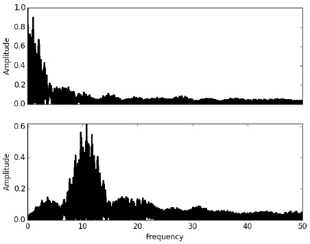
Fig. 3 Periodogram of all the available light curves of BO Lyn. Top: the window function. Bottom: the obtained periodogram.
Once the whole time string was analyzed the period was utilized as a seed period, which was taken to calculate the number of cycles, E. A least squares fit of TMAX vs. E was implemented giving as output the refined period and the corrected initial epoch T0 of the ephemerides equation, as well as the error parameters. The resultant equation is the following:
4.2. Minimization of the Standard Deviation of the O-C Residuals (MSDR)
The second method utilizes as criteria of good-ness, the minimization of the standard deviation of the O-C residuals (MSDR).
We implemented a method based on the O-C standard deviation minimization analogous to the idea proposed by Stellingwerf (1978) for period determination by phase dispersion minimization. We considered the set of TMAX listed in Table 3 in our analysis. The mean period was determined through the differences of two or three times of maxima that were observed on the same night and the associated standard deviation. Given the standard deviation and the period we determined, we swept between these limits calculating 5000 steps which gives the sufficient accuracy provided by the time span of the observations. The obtained precision of one millionth provides the new period and the limits for the iteration (Figure 4). In each iteration, the O-C standard deviation was calculated. We chose as the best period that which showed the minimum standard deviation. The resulting equation is:

The previous methods gave basically the same result. Therefore, it can be seen that the O-C residuals show a sinusoidal behavior. This pattern in the O-C diagram is usually related with the light-travel time effect (LTT). In view of this, the O-C residuals were analyzed in Period04 and fitted with an equation of the following type:
The result is shown in Figure 5 and the elements of the fit are listed in Table 4.
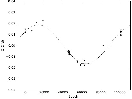
Table 4 Equation parameters for the sinusoidal fit of the O-C residuals.
| Value | Period04 & MSDR | PDDM |
|---|---|---|
| Z | 1.17 × 10⁻³ | −1.67 × 10⁻² |
| Ω | 9.85 × 10⁻⁶ | 1.18 × 10⁻⁵ |
| A | 1.76 × 10⁻² | 1.68 × 10⁻² |
| Φ | 1.14 × 10⁻¹ | 2.39 × 10⁻¹ |
| ZErr | 4.25 × 10⁻⁴ | 3.62 × 10⁻⁴ |
| ΩErr | 2.43 × 10⁻⁷ | 2.31 × 10⁻⁷ |
| AErr | 5.82 × 10⁻⁴ | 4.89 × 10⁻⁴ |
| ΦErr | 7.81 × 10⁻³ | 1.65 × 10⁻² |
| Residuals | 2.00 × 10⁻³ | 1.9 × 10⁻³ |
4.3. Period determination through an O-C differences minimization (PDDM)
In the third procedure, we implemented a method based on the idea of searching the minimization of the chord length which links all the points in the O-C diagram for different values of the periods, looking for the best period which corresponds to the minimum chord length. With this idea in mind, we tried to obtain the smoothest curve. Since we were dealing with the classical O-C diagram, we plotted the time in the x-axis and the O-C values in the y-axis. Since in the x-axis distances are constant, we just concentrated on the change in the distance in the y-axis in each diagram, generated by one period. Once the difference was calculated for each period, the minimum one indicated, at this stage, the best period (period determination through an O-C differences minimization PDDM). We considered the set of Tmax listed in Table 3 in our analysis. Given the mean period determined from the consecutive times of maxima and the associated standard deviation, (0.0936 days and 0.0027 days), we calculated values of epoch and O-C by sweeping the period in the range provided by the standard deviation limits, 0.091 to 0.096 days, calculating 5 × 10⁶ steps, a number fixed by the the difference of the deviation limits and the desired precision of one billionth. This provided the new period for the minimum difference (Figure 6). The T0 time used for the present analysis was the one of the 2016 observation run, 2457412.8196, because we are certain of its precision.

As a result we determined the linear ephemerides equation as:
Figure 7 shows the O-C diagram for the ephemerides equation found by the above method (PDDM).

Assuming the wave behavior as a part of the physics in the system, we adjusted a sinusoidal function to the O-C, performing a fitting using Levenberg-Marquardt Algorithm for the best 1,000 O-C lengths. This would be, in this particular case, another way of finding the best period and, at the same time, the sinusoidal function which is similar to the one assumed in the second method. The parameters which best represents the system are listed in Table 4. The parameter used to prove the goodness of the adjustment is the residual sum of squares RSS. Then, we plotted the periods of the best O-C lengths vs. the RSS value of every fit, Figure 8.

After this, the ephemeris equation was set as:
As we can see, only one frequency explains this sinusoidal behavior. The parameters are presented in Table 4 and are shown schematically in Figure 9. This frequency corresponds to a period of 7,779.83 days or 21.49 years.

4.4. (O-C) Discussion
BO Lyn was discovered relatively recently and has been scarcely observed. The whole sample of times of maximum light contains only 34 unevenly distributed entries.
As can be seen, the parameters of the equations obtained with the light curves analyses and the standard deviation minimization for the times of maxima give the same results. This confirms the results among themselves since both solutions converge to the same period. Then in both cases a sinusoidal behavior can be seen. The third method, PDDM, with a completely different approach, gives basically the same results.
After a quick review of the most conspicuous and well-studied HADS stars, the majority (nine) have increasing period changes and only a few (four), the opposite. What we have found in BO Lyn is that it is a star in a stable evolutionary stage.
With respect to its amplitude, a variation in the light curves was suggested by Kinman (1998), and later Hintz et al. (2005) suggested that this could be due to two probable secondary frequencies in the pulsation modes. In our analysis we can explain the behavior of the star with only one pulsational period and an orbital period.
Continued monitoring of times of maximum will be crucial, and such observations are encouraged.
5. Physical parameters
Physical parameters can be obtained using the advantages given by Strömgren photometry with calibrations made by Nissen (1988) for the A and F stars or by Shobbrook (1984), for earlier spectral types. These calibrations are described in detail in Peña et al. (2002).
The evaluation of the reddening was done by first establishing to which spectral class the stars belong. As a primary criterion the location of the stars in the [m1] − [c1] diagram of the classical textbook of Golay (1974) (Figure 10) or the results derived for the open cluster α Per (Peña & Sareyan, 2006) were employed. As can be seen in this figure, the spectral type of BO Lyn varies between A5 and A8. There has been until now, no assignment of a spectral type for BO Lyn. Once a spectral class is assigned, we can choose the prescription for unreddening which, for the spectral type of BO Lyn, is that of Nissen (1988).

5.1. Data Acquisition and Reduction at SPM
The observational pattern as well as the reduction procedure have been employed at the SPM Observatory since 1986 and hence have been described many times. A detailed description of the method-ology can be found in Peña et al. (2007). During the three nights of observations the following procedure was utilized: each measurement consisted of at least five ten-second integrations of each star and one ten-second integration of the sky for the uvby filters and the narrow and wide filters that define Hβ. It is important to emphasize here that the transformation coefficients for the observed season (Table 5) and the season errors were evaluated using the ninety-one observed standard stars. These uncertainties were calculated through the differences in magnitude and colors for (V, b − y, m 1, c 1 and β) which were (0.054, 0.012, 0.019, 0.025, 0.012), respectively. We emphasize the large range of the standard stars in the magnitude and color values: V: (5.62, 8.0); (b − y):(-0.09, 0.88); m 1:(-0.09, 0.67); c 1:(-0.024, 1.32) and β:(2.495, 2.90).
Table 5 Transformation coefficients obtained for the 2016 season.
| Coefficient | B | D | F | J | H | I | L |
|---|---|---|---|---|---|---|---|
| value | 0.031 | 1.008 | 1.031 | −0.004 | 1.015 | 0.159 | −1.362 |
| σ | 0.028 | 0.003 | 0.015 | 0.017 | 0.005 | 0.004 | 0.060 |
Table 6 lists the photometric values of the observed star. In this table Column 1 contains the time of the observation in HJD, Columns 2 to 5 the Strömgren values V, (b −y), m 1 and c 1, respectively; Column 6 lists β, whereas Columns 7 to 9 list the unreddened indexes [m1], [c1] and [u-b] derived from the observations. Unfortunately in none of the SPM observations (two nights) a time of maximum light was reached, although the observations were almost long enough to completely cover the whole pulsation cycle.
Table 6 uvby-β photoelectric photometry of BO Lyn.
| HJD | V | (b − y) | m 1 | c 1 | β | [m1] | [c1] | [u − b] |
|---|---|---|---|---|---|---|---|---|
| -2457000.00 | ||||||||
| 399.8477 | 11.875 | 0.130 | 0.195 | 0.928 | 2.706 | 0.237 | 0.902 | 1.375 |
| 399.8506 | 11.865 | 0.160 | 0.154 | 0.952 | 2.754 | 0.205 | 0.920 | 1.330 |
| 399.8546 | 11.897 | 0.149 | 0.186 | 0.872 | 2.743 | 0.234 | 0.842 | 1.310 |
| 399.8567 | 11.894 | 0.162 | 0.180 | 0.865 | 2.791 | 0.232 | 0.833 | 1.296 |
| 399.8591 | 11.901 | 0.172 | 0.169 | 0.881 | 2.774 | 0.224 | 0.847 | 1.295 |
| 399.8617 | 11.937 | 0.160 | 0.167 | 0.893 | 2.804 | 0.218 | 0.861 | 1.297 |
| 399.8638 | 11.944 | 0.166 | 0.177 | 0.881 | 2.751 | 0.230 | 0.848 | 1.308 |
| 399.8662 | 11.974 | 0.164 | 0.157 | 0.882 | 2.683 | 0.209 | 0.849 | 1.268 |
| 399.8706 | 11.980 | 0.193 | 0.139 | 0.877 | 2.730 | 0.201 | 0.838 | 1.240 |
| 399.8728 | 11.974 | 0.210 | 0.123 | 0.877 | 2.695 | 0.190 | 0.835 | 1.215 |
| 399.8747 | 11.999 | 0.195 | 0.157 | 0.833 | 2.682 | 0.219 | 0.794 | 1.233 |
| 399.8768 | 12.012 | 0.192 | 0.167 | 0.824 | 2.664 | 0.228 | 0.786 | 1.242 |
| 399.8790 | 12.015 | 0.206 | 0.135 | 0.856 | 2.731 | 0.201 | 0.815 | 1.217 |
| 399.8809 | 12.056 | 0.155 | 0.222 | 0.802 | 2.691 | 0.272 | 0.771 | 1.314 |
| 399.8846 | 12.076 | 0.157 | 0.215 | 0.784 | 2.675 | 0.265 | 0.753 | 1.283 |
| 399.8864 | 12.064 | 0.174 | 0.190 | 0.812 | 2.713 | 0.246 | 0.777 | 1.269 |
| 399.8895 | 12.057 | 0.188 | 0.178 | 0.791 | 2.698 | 0.238 | 0.753 | 1.230 |
| 399.8926 | 12.059 | 0.196 | 0.155 | 0.830 | 2.694 | 0.218 | 0.791 | 1.226 |
| 399.8946 | 12.061 | 0.181 | 0.171 | 0.823 | 2.715 | 0.229 | 0.787 | 1.245 |
| 399.8966 | 11.964 | 0.253 | 0.121 | 0.717 | 2.739 | 0.202 | 0.666 | 1.070 |
| 399.9008 | 11.956 | 0.247 | 0.118 | 0.739 | 2.730 | 0.197 | 0.690 | 1.084 |
| 399.9027 | 11.962 | 0.232 | 0.115 | 0.791 | 2.708 | 0.189 | 0.745 | 1.123 |
| 399.9049 | 11.950 | 0.224 | 0.139 | 0.751 | 2.719 | 0.211 | 0.706 | 1.128 |
| 399.9073 | 11.939 | 0.205 | 0.148 | 0.795 | 2.715 | 0.214 | 0.754 | 1.181 |
| 399.9093 | 11.907 | 0.221 | 0.124 | 0.792 | 2.717 | 0.195 | 0.748 | 1.137 |
| 399.9114 | 11.955 | 0.173 | 0.162 | 0.869 | 2.777 | 0.217 | 0.834 | 1.269 |
| 399.9157 | 11.916 | 0.167 | 0.159 | 0.878 | 2.731 | 0.212 | 0.845 | 1.269 |
| 399.9176 | 11.918 | 0.161 | 0.173 | 0.907 | 2.811 | 0.225 | 0.875 | 1.324 |
| 399.9193 | 11.878 | 0.168 | 0.151 | 0.913 | 2.792 | 0.205 | 0.879 | 1.289 |
| 399.9208 | 11.911 | 0.135 | 0.190 | 0.912 | 2.743 | 0.233 | 0.885 | 1.351 |
| 399.9224 | 11.857 | 0.163 | 0.163 | 0.891 | 2.757 | 0.215 | 0.858 | 1.289 |
| 399.9240 | 11.840 | 0.153 | 0.160 | 0.950 | 2.742 | 0.209 | 0.919 | 1.337 |
| 399.9257 | 11.828 | 0.151 | 0.163 | 0.925 | 2.777 | 0.211 | 0.895 | 1.317 |
| 399.9276 | 11.833 | 0.142 | 0.176 | 0.911 | 2.770 | 0.221 | 0.883 | 1.325 |
| 401.9013 | 11.842 | 0.155 | 0.171 | 0.918 | 2.764 | 0.221 | 0.887 | 1.328 |
| 401.9033 | 11.838 | 0.159 | 0.164 | 0.923 | 2.796 | 0.215 | 0.891 | 1.321 |
| 401.9052 | 11.845 | 0.180 | 0.146 | 0.939 | 2.799 | 0.204 | 0.903 | 1.310 |
| 401.9070 | 11.863 | 0.167 | 0.166 | 0.901 | 2.773 | 0.219 | 0.868 | 1.306 |
| 401.9086 | 11.879 | 0.157 | 0.177 | 0.913 | 2.789 | 0.227 | 0.882 | 1.336 |
| 401.9103 | 11.888 | 0.169 | 0.151 | 0.934 | 2.779 | 0.205 | 0.900 | 1.310 |
| 401.9135 | 11.909 | 0.152 | 0.195 | 0.878 | 2.730 | 0.244 | 0.848 | 1.335 |
| 401.9152 | 11.897 | 0.171 | 0.173 | 0.895 | 2.794 | 0.228 | 0.861 | 1.316 |
| 401.9168 | 11.914 | 0.187 | 0.144 | 0.909 | 2.774 | 0.204 | 0.872 | 1.279 |
| 401.9187 | 11.927 | 0.173 | 0.173 | 0.895 | 2.794 | 0.228 | 0.860 | 1.317 |
| 401.9207 | 11.921 | 0.189 | 0.164 | 0.866 | 2.783 | 0.224 | 0.828 | 1.277 |
| 401.9227 | 11.951 | 0.182 | 0.164 | 0.875 | 2.788 | 0.222 | 0.839 | 1.283 |
| 401.9245 | 11.964 | 0.185 | 0.153 | 0.893 | 2.806 | 0.212 | 0.856 | 1.280 |
| 401.9264 | 11.961 | 0.202 | 0.133 | 0.881 | 2.766 | 0.198 | 0.841 | 1.236 |
| 401.9301 | 11.969 | 0.195 | 0.174 | 0.855 | 2.746 | 0.236 | 0.816 | 1.289 |
| 401.9319 | 11.983 | 0.187 | 0.184 | 0.825 | 2.753 | 0.244 | 0.788 | 1.275 |
| 401.9337 | 11.992 | 0.199 | 0.169 | 0.829 | 2.802 | 0.233 | 0.789 | 1.255 |
| 401.9362 | 12.000 | 0.204 | 0.162 | 0.814 | 2.719 | 0.227 | 0.773 | 1.228 |
| 401.9378 | 12.005 | 0.217 | 0.146 | 0.822 | 2.753 | 0.215 | 0.779 | 1.209 |
| 401.9395 | 12.015 | 0.208 | 0.155 | 0.834 | 2.743 | 0.222 | 0.792 | 1.236 |
| 401.9411 | 12.039 | 0.195 | 0.159 | 0.827 | 2.728 | 0.221 | 0.788 | 1.231 |
| 401.9430 | 12.033 | 0.218 | 0.147 | 0.790 | 2.769 | 0.217 | 0.746 | 1.180 |
| 401.9450 | 12.030 | 0.231 | 0.121 | 0.825 | 2.769 | 0.195 | 0.779 | 1.169 |
| 401.9469 | 12.039 | 0.212 | 0.133 | 0.852 | 2.734 | 0.201 | 0.810 | 1.211 |
| 401.9509 | 12.033 | 0.231 | 0.130 | 0.837 | 2.672 | 0.204 | 0.791 | 1.199 |
| 401.9526 | 12.046 | 0.219 | 0.141 | 0.812 | 2.670 | 0.211 | 0.768 | 1.190 |
| 401.9547 | 12.058 | 0.193 | 0.159 | 0.829 | 2.784 | 0.221 | 0.790 | 1.232 |
| 401.9567 | 12.031 | 0.210 | 0.146 | 0.811 | 2.770 | 0.213 | 0.769 | 1.195 |
| 401.9586 | 12.025 | 0.203 | 0.151 | 0.830 | 2.773 | 0.216 | 0.789 | 1.221 |
| 401.9610 | 12.010 | 0.212 | 0.147 | 0.810 | 2.758 | 0.215 | 0.768 | 1.197 |
| 401.9631 | 12.015 | 0.183 | 0.185 | 0.791 | 2.770 | 0.244 | 0.754 | 1.242 |
| 401.9652 | 11.990 | 0.187 | 0.176 | 0.818 | 2.791 | 0.236 | 0.781 | 1.252 |
| 401.9677 | 11.959 | 0.213 | 0.137 | 0.845 | 2.779 | 0.205 | 0.802 | 1.213 |
| 401.9697 | 11.971 | 0.170 | 0.169 | 0.836 | 2.753 | 0.223 | 0.802 | 1.249 |
| 401.9714 | 11.921 | 0.190 | 0.156 | 0.863 | 2.747 | 0.217 | 0.825 | 1.259 |
| 401.9735 | 11.913 | 0.188 | 0.147 | 0.868 | 2.828 | 0.207 | 0.830 | 1.245 |
| 401.9772 | 11.891 | 0.185 | 0.148 | 0.885 | 2.779 | 0.207 | 0.848 | 1.262 |
| 401.9791 | 11.885 | 0.166 | 0.176 | 0.866 | 2.751 | 0.229 | 0.833 | 1.291 |
| 401.9812 | 11.846 | 0.166 | 0.154 | 0.920 | 2.781 | 0.207 | 0.887 | 1.301 |
| 401.9832 | 11.828 | 0.171 | 0.150 | 0.919 | 2.817 | 0.205 | 0.885 | 1.294 |
| 401.9852 | 11.814 | 0.179 | 0.132 | 0.948 | 2.810 | 0.189 | 0.912 | 1.291 |
| 401.9869 | 11.813 | 0.166 | 0.144 | 0.940 | 2.833 | 0.197 | 0.907 | 1.301 |
5.2. Physical Parameter Determination
The application of the above mentioned numerical unreddening packages gave the results listed in Table 7 for BO Lyn. This table lists, in the first column, the HJD. Subsequent columns present the reddening, the unreddened indexes, the unreddened magnitude, the absolute magnitude, the distance modulus, and the distance. Mean values were calculated for E(b − y), the distance modulus (DM) and the distance for two cases: (i) the whole data sample and (ii) in phase limits between 0.3 and 0.8, which is customary for pulsating stars to avoid the maximum. We obtained, for the whole cycle, values of 0.020 ± 0.021; 10.7 ± 0.9 and 1497 ± 756 for E(b − y), DM and distance (in pc), respectively, whereas for the mentioned phase limits we obtained, 0.022 ±0.022; 10.5 ±0.8 and 1383 ±702 respectively. The uncertainty is merely the standard deviation. In the case of the reddening, most of the values for the spectral type F of BO Lyn produced negative values which is unphysical. In those cases we forced the reddening to be zero in which case the (b − y) index is the same. If the negative values are included, the mean E(b − y) is 0.009 ± 0.038.
Table 7 Reddening and unreddened parameters of BO Lyn.
| HJD | E(b − y) | (b − y) 0 | m 0 | c 0 | Hβ | V 0 | M V | DM | d(pc) |
|---|---|---|---|---|---|---|---|---|---|
| -2457000.00 | |||||||||
| 401.9832 | .052 | .119 | .166 | .909 | 2.817 | 11.60 | 1.76 | 9.84 | 928 |
| 399.9176 | .036 | .125 | .184 | .900 | 2.811 | 11.76 | 1.78 | 9.98 | 990 |
| 401.9852 | .058 | .121 | .149 | .936 | 2.810 | 11.57 | 1.40 | 10.17 | 1080 |
| 401.9245 | .055 | .130 | .170 | .882 | 2.806 | 11.73 | 1.83 | 9.89 | 952 |
| 399.8617 | .028 | .132 | .176 | .887 | 2.804 | 11.81 | 1.80 | 10.01 | 1005 |
| 401.9337 | .059 | .140 | .187 | .817 | 2.802 | 11.74 | 2.35 | 9.39 | 754 |
| 401.9052 | .049 | .131 | .161 | .929 | 2.799 | 11.63 | 1.31 | 10.32 | 1159 |
| 401.9033 | .024 | .135 | .171 | .918 | 2.796 | 11.73 | 1.41 | 10.32 | 1160 |
| 401.9152 | .032 | .139 | .183 | .889 | 2.794 | 11.76 | 1.63 | 10.13 | 1060 |
| 401.9187 | .034 | .139 | .183 | .888 | 2.794 | 11.78 | 1.63 | 10.15 | 1070 |
| 399.9193 | .029 | .139 | .160 | .907 | 2.792 | 11.75 | 1.44 | 10.31 | 1154 |
| 399.8567 | .017 | .145 | .185 | .862 | 2.791 | 11.82 | 1.86 | 9.96 | 982 |
| 401.9652 | .038 | .149 | .187 | .810 | 2.791 | 11.83 | 2.28 | 9.55 | 811 |
| 401.9086 | .015 | .142 | .182 | .910 | 2.789 | 11.81 | 1.40 | 10.41 | 1210 |
| 401.9227 | .036 | .146 | .175 | .868 | 2.788 | 11.80 | 1.73 | 10.07 | 1034 |
| 401.9547 | .039 | .154 | .171 | .821 | 2.784 | 11.89 | 2.08 | 9.81 | 917 |
| 401.9207 | .038 | .151 | .175 | .858 | 2.783 | 11.76 | 1.73 | 10.03 | 1012 |
| 401.9812 | .019 | .147 | .160 | .916 | 2.781 | 11.77 | 1.21 | 10.55 | 1288 |
| 401.9103 | .022 | .147 | .157 | .930 | 2.779 | 11.80 | 1.06 | 10.74 | 1404 |
| 401.9677 | .057 | .156 | .154 | .834 | 2.779 | 11.72 | 1.86 | 9.86 | 935 |
| 401.9772 | .033 | .152 | .158 | .878 | 2.779 | 11.75 | 1.50 | 10.25 | 1122 |
| 399.9114 | .017 | .156 | .167 | .866 | 2.777 | 11.88 | 1.61 | 10.27 | 1130 |
| 399.9257 | .001 | .150 | .163 | .925 | 2.777 | 11.82 | 1.11 | 10.71 | 1389 |
| 399.8591 | .015 | .157 | .174 | .878 | 2.774 | 11.84 | 1.46 | 10.37 | 1188 |
| 401.9168 | .033 | .154 | .154 | .902 | 2.774 | 11.77 | 1.21 | 10.56 | 1296 |
| 401.9070 | .011 | .156 | .169 | .899 | 2.773 | 11.81 | 1.27 | 10.55 | 1287 |
| 401.9586 | .040 | .163 | .163 | .822 | 2.773 | 11.85 | 1.91 | 9.95 | 976 |
| 399.9276 | .000 | .142 | .176 | .911 | 2.770 | 11.83 | 1.13 | 10.70 | 1382 |
| 401.9567 | .043 | .167 | .159 | .802 | 2.770 | 11.85 | 2.03 | 9.81 | 918 |
| 401.9631 | .014 | .169 | .189 | .788 | 2.770 | 11.95 | 2.21 | 9.74 | 889 |
| 401.9430 | .048 | .170 | .161 | .780 | 2.769 | 11.83 | 2.21 | 9.62 | 840 |
| 401.9450 | .065 | .166 | .140 | .812 | 2.769 | 11.75 | 1.89 | 9.86 | 938 |
| 401.9264 | .039 | .163 | .145 | .873 | 2.766 | 11.79 | 1.34 | 10.45 | 1232 |
| 401.9013 | .000 | .155 | .171 | .918 | 2.764 | 11.84 | .98 | 10.86 | 1489 |
| 401.9610 | .035 | .177 | .158 | .803 | 2.758 | 11.86 | 1.86 | 10.00 | 998 |
| 399.9224 | .000 | .163 | .163 | .891 | 2.757 | 11.86 | 1.12 | 10.74 | 1405 |
| 399.8506 | .000 | .160 | .154 | .952 | 2.754 | 11.86 | .53 | 11.34 | 1851 |
| 401.9319 | .008 | .179 | .186 | .823 | 2.753 | 11.95 | 1.66 | 10.29 | 1144 |
| 401.9378 | .038 | .179 | .157 | .814 | 2.753 | 11.84 | 1.68 | 10.16 | 1076 |
| 401.9697 | .000 | .170 | .169 | .836 | 2.753 | 11.97 | 1.56 | 10.41 | 1209 |
| 399.8638 | .000 | .166 | .177 | .881 | 2.751 | 11.94 | 1.12 | 10.82 | 1458 |
| 401.9791 | .000 | .166 | .176 | .866 | 2.751 | 11.89 | 1.26 | 10.63 | 1334 |
| 401.9714 | .010 | .180 | .159 | .861 | 2.747 | 11.88 | 1.23 | 10.65 | 1347 |
| 401.9301 | .013 | .182 | .178 | .852 | 2.746 | 11.91 | 1.29 | 10.62 | 1332 |
| 399.8546 | .000 | .149 | .186 | .872 | 2.743 | 11.90 | 1.09 | 10.80 | 1447 |
| 399.9208 | .000 | .135 | .190 | .912 | 2.743 | 11.91 | .73 | 11.18 | 1719 |
| 401.9395 | .022 | .186 | .162 | .830 | 2.743 | 11.92 | 1.44 | 10.49 | 1250 |
| 399.9240 | .000 | .153 | .160 | .950 | 2.742 | 11.84 | .38 | 11.46 | 1961 |
| 399.8966 | .052 | .201 | .137 | .707 | 2.739 | 11.74 | 2.42 | 9.32 | 730 |
| 401.9469 | .021 | .191 | .139 | .848 | 2.734 | 11.95 | 1.09 | 10.86 | 1483 |
| 399.8790 | .014 | .192 | .139 | .853 | 2.731 | 11.96 | .98 | 10.97 | 1564 |
| 399.9157 | .000 | .167 | .159 | .878 | 2.731 | 11.92 | .79 | 11.13 | 1682 |
| 399.8706 | .002 | .191 | .140 | .877 | 2.730 | 11.97 | .77 | 11.20 | 1737 |
| 399.9008 | .042 | .205 | .131 | .731 | 2.730 | 11.77 | 2.01 | 9.76 | 895 |
| 401.9135 | .000 | .152 | .195 | .878 | 2.730 | 11.91 | .76 | 11.15 | 1695 |
| 401.9411 | .000 | .195 | .159 | .827 | 2.728 | 12.04 | 1.17 | 10.86 | 1489 |
| 399.9049 | .016 | .208 | .144 | .748 | 2.719 | 11.88 | 1.64 | 10.23 | 1114 |
| 401.9362 | .000 | .204 | .162 | .814 | 2.719 | 12.00 | 1.07 | 10.93 | 1531 |
| 399.9093 | .015 | .206 | .129 | .789 | 2.717 | 11.84 | 1.22 | 10.62 | 1333 |
| 399.8946 | .000 | .181 | .171 | .823 | 2.715 | 12.06 | .87 | 11.19 | 1730 |
| 399.9073 | .000 | .205 | .148 | .795 | 2.715 | 11.94 | 1.13 | 10.81 | 1451 |
| 399.8864 | .000 | .174 | .190 | .812 | 2.713 | 12.06 | .91 | 11.15 | 1701 |
| 399.9027 | .020 | .212 | .121 | .787 | 2.708 | 11.88 | .95 | 10.93 | 1532 |
| 399.8477 | .000 | .130 | .195 | .928 | 2.706 | 11.88 | -.44 | 12.32 | 2909 |
| 399.8895 | .000 | .188 | .178 | .791 | 2.698 | 12.06 | .60 | 11.46 | 1955 |
| 399.8728 | .000 | .210 | .123 | .877 | 2.695 | 11.97 | -.40 | 12.38 | 2986 |
| 399.8926 | .000 | .196 | .155 | .830 | 2.694 | 12.06 | .04 | 12.02 | 2537 |
| 399.8809 | .000 | .155 | .222 | .802 | 2.691 | 12.06 | .20 | 11.86 | 2351 |
| 399.8662 | .000 | .164 | .157 | .882 | 2.683 | 11.97 | -.98 | 12.95 | 3892 |
| 399.8747 | .000 | .195 | .157 | .833 | 2.682 | 12.00 | -.49 | 12.48 | 3140 |
| 399.8846 | .000 | .157 | .215 | .784 | 2.675 | 12.08 | -.19 | 12.27 | 2838 |
| 401.9509 | .000 | .231 | .130 | .837 | 2.672 | 12.03 | -.89 | 12.93 | 3847 |
| 401.9526 | .000 | .219 | .141 | .812 | 2.670 | 12.05 | -.68 | 12.72 | 3506 |
| 399.8768 | .000 | .192 | .167 | .824 | 2.664 | 12.01 | -1.02 | 13.04 | 4048 |
If the photometric system is well-defined and calibrated, it provides an efficient way to investigate physical conditions such as effective temperature and surface gravity via a direct comparison of the unreddened indexes with the theoretical models. These calibrations have already been described and used in previous analyses (Peña & Peniche; 1994; Peña & Sareyan, 2006).
A comparison between theoretical models, such as those of Lester, Gray & Kurucz (1986), hereinafter LGK86 and intermediate or wide band photometry obtained for the stars allows a direct comparison. LGK86 calculated grids for stellar atmospheres for G, F, A, B and O stars with different values of [Fe/H] in a temperature range from 5500 up to 50 000 K. The surface gravities vary approximately from the main sequence values to the limit of the radiation pressure in 0.5 intervals in log g. A comparison be-tween the photometric unreddened indexes (b − y)0 and c0 obtained for each star with the models al-lowed us to determine the effective temperature Te and surface gravity log g.
In order to locate our unreddened points in the theoretical grids of LGK86, a metallicity had to be assumed. LGK86 calculated their outputs for several metallicities. Particularly in the case of BO Lyn, for which we determined a mean metallicity of [Fe/H] = −0.39 ± 0.31, there are two applicable models, either [Fe/H] = 0.0 or −0.5. We tested both since our determined mean metallicity of [Fe/H] = −0.39 ± 0.31 lies in between. To diminish the noise and to see the variation of the star in phase, mean values of the unreddened colors were calculated in phase bins of 0.1 starting at 0.05. As can be seen in Figure 11, for the case of [Fe/H] = −0.5, the effective temperature varies between 7000 K and 7700 K; the surface gravity varies between 3.4 and 3.9. Table 8 lists these values. Column 1 shows the phase, Columns 2 and 3 list the temperature obtained from the plot for each [Fe/H] value; Column 4, the mean value and Column 5, the standard deviation for a [Fe/H] = −0.5 metallicity. Column 6 lists the effective temperature obtained from the theoretical relation reported by Rodriguez (1989) based on a relation of Petersen & Jorgensen (1972, hereinafter P&J) Te = 6850 + 1250 × (β − 2.684)/0.144 for each value and averaged in the corresponding phase bin. The last column lists the surface gravity log g from the plot.
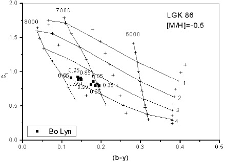
Fig. 11 Location of the unreddened points of BO Lyn (dots) in the LGK86 grids. The numbers indicate the phase.
Table 8 Effective temperature of BO Lyn.
| Phase | T e | T e | Mean | OP&J | log g |
|---|---|---|---|---|---|
| [Fe/H] | 0.0 | -0.5 | -0.5 | -0.5 | |
| 0.05 | 7300 | 7100 | 7200 | 7251 | 3.4 |
| 0.15 | 7400 | 7200 | 7300 | 7235 | 3.8 |
| 0.25 | 7300 | 7200 | 7250 | 7259 | 3.8 |
| 0.35 | 7200 | 7000 | 7100 | 7234 | 3.6 |
| 0.45 | 7400 | 7500 | 7450 | 7494 | 3.7 |
| 0.55 | 7800 | 7500 | 7650 | 7582 | 3.8 |
| 0.65 | 8000 | 7700 | 7850 | 7781 | 3.9 |
| 0.75 | 7800 | 7500 | 7650 | 7469 | 3.7 |
| 0.85 | 7700 | 7400 | 7550 | 7642 | 3.7 |
| 0.95 | 7700 | 7400 | 7500 | 7569 | 3.5 |
5.3. Physical Parameter Discussion
New observations in uvby −β photoelectric photometry were carried out on the HADS star BO Lyn. From this uvby −β photoelectric photometry we determined first its spectral type, varying between A5V and A8V. From Nissen’s (1988) calibrations the reddening was determined as well as the unreddened indexes. These served to obtain the physical characteristics of this star, log Te, in the range from 7000 K to 7700 K and log g from 3.2 to 3.6, using two methods: (1) from the location of the unreddened indexes in the LGK86 grids and (2) through the theoretical relation (Petersen et al., 1972). They are similar within the error bars, and give a good idea of the star’s behavior. Furthermore, when mean values are obtained from the two closest metallicity values, the result is closer to the obtained theoretical value.
6. Discussion
According to Rodriguez & Breger (2001) “only 14 % of the known δ Scuti stars are part of binary or multiple stellar systems Only five variables are fainter than V = 10.0.... Hence, multiplicity is catalogued for 22 of all the δ Scuti known up 10. 0. This percentage is very low because more than 50% of the stars are expected to be members of multiple systems”. They later state that “pulsating stars in eclipsing binaries are important for accurate determinations of fundamental stellar parameters and the study of tidal effects on the pulsations.... During the last two decades, unusual changes in the light curves have been detected, leading to a number of different interpretations...”
They later say that “pulsation provides an additional method to detect multiplicity through a study of the light-time effects in a binary system. This method generally favors high-amplitude variables with only one or two pulsation periods (which tend to be radial). Several decades of measurements are usually required to study these (O-C) residuals in the times of maxima”.
At that time they listed, in their Table 4, only six stars with known orbital periods. Since then, with a longer time basis for those stars, and for an increased number of measured times of maximum, a better definition of their orbital elements is available. There have been numerous studies of HADS stars with this purpose. For example, Boonyarak et al. (2011) carried out a study devoted to the analysis of the stability of fourteen stars of this type. Many other authors carried out analyses on a star-by-star basis. Some of the HADS stars show a behavior of the O-C residuals compatible with the light-travel time effect that is expected for the binaries AD CMi, KZ Hya, AN Lyn, BE Lyn, SZ Lyn, BP Peg, BS Aqr, CY Aqr, among others; whereas there are some stars that, on the contrary, are varying with one period and its harmonics and do not show a light-travel time effect. To this category, according to Boonyarak et al., (2011) belong GP And, AZ CMi, AE UMa, RV Ari, DY Her, DH Peg.
In the present study we have demonstrated that BO Lyn is pulsating with one stable varying period whose O-C residuals show a sinusoidal pattern compatible with a light-travel time effect. In relation to this topic, it is interesting to mention that in the excellent discussion of Templeton (2005), he states that: “In all cases except SZ Lyn, the period of the purported binarity is close to that of the duration of the (O-C) measurements, making it difficult to prove that the signal is truly sinusoidal. A sinusoidal interpretation is only reliable when multiple cycles are recorded, as in SZ Lyn. While the binary hypothesis is certainly possible in most of these cases, conclusive proof will not be available for years or even decades to come. Continued monitoring of times of maximum will be crucial, and such observations are encouraged. In the meantime, however, other possible interpretations of their behavior must also be explored”.
We feel that the results presented in this paper fulfill Templeton’s (2005) requirement that “a sinusoidal interpretation is only reliable when multiple cycles are recorded”.

