


 nueva página del texto (beta)
 Inglés (pdf)
 Artículo en XML
 Referencias del artículo
 Enviar artículo por email
 Citado por SciELO
  Similares en
SciELO
Similares en
SciELO 
 Permalink
1. Introduction
In Cisneros et al. I (2015) equilibrium figures were obtained from a self-gravitating homogeneous liquid mass endowed with an internal motion of differential vorticity, whose surface equation was that of either a distorted ellipsoid or a distorted spheroid; however, as we noticed a posteriori, the figures, called ellipsoidal and spheroidal after Jeans (1920), were erroneously deduced, although their qualitative features remained more or less unaffected (see § 5.1). In the current paper, we investigate the equilibrium of a heterogeneous model consisting of two concentric homogeneous spheroidal masses of different density, the ‘nucleus’ and the ‘atmosphere’ (whose semi-axes are not correlated) through a simple and precise rotation law. Affixing sub indexes n and a to the pertinent quantities, the body’s relative density, (ρn− ρa)/ρa , is denoted by ε, with ρn > ρa, so that the distribution of density is somewhat closer to that prevailing in real stars. The quantities in our development are normalized as explained in Cisneros et al. I (2015).
2.Bernoulli’s theorem, the classical homogeneous figures and ours
Before going on with our heterogeneous model, we wish to discuss Bernoulli’s theorem as is commonly employed for obtaining the classical homogeneous figures (Lyttleton 1953; Dryden 1956), particularly the Dedekind ellipsoids which, along with our models, are static. The steady-state equations of motion for a self-gravitating fluid are
where v is the velocity field, V is the potential and p is the pressure. These equations can also be written as
For a streamline (tangent to v) we get, after taking the dot product of v in the first equation (2),
that is
k being constant on a streamline. Commonly, k changes from one streamline to another, being an overall constant only when rot v = 0. The changes in k are dictated by [cf. equations (2) and (4)]
The Maclaurin and Jacobi figures are characterized by the rotational velocity field
where ω is the constant angular velocity. We can see that relation (6) satisfies the continuity equation div v = 0. According to equation (6), the k in Bernoulli’s equation is given by
that is
From which we deduce
c being any constant. Therefore, Bernoulli’s equation (4) becomes
which agrees with the well-known equation.1
While the Jacobi and the Maclaurin figures rotate as a rigid body, a Dedekind ellipsoid (1, e2, e3 are the major, middle, and minor semi-axes) remains fixed in space, its equilibrium being due to an internal motion of uniform vorticity ζ, its velocity field being
We can convince ourselves that V is tangent to ellipses x2 + y2/e22 = const.. Hence, streamlines are ellipses perpendicular to the z-axis. For ζ constant, the velocity field satisfies the continuity equation, and k obeys the relation
so that
The solution of the partial differential equations (13) is
where c is an arbitrary constant. In this case, Bernoulli’s equation
reduces to
This is essentially equation (10) for obtaining the Jacobi ellipsoids if we put
a known result that establishes the equivalence between Jacobi’s angular velocity and Dedekind’s vorticity (Chandrasekhar 1969). Of course, if we had assumed from the beginning that k = const., it would have been impossible to reach equation (15).
2.1. General Case with Cylindrical Symmetry
Each fluid point rotates, now, with non-constant angular velocity ω. The velocity field is given again by
but the continuity equation leads, presently, to
or
which means that, generally, the angular velocity must be a function of the kind
Assuming, additionally, that the velocity field is symmetric about the z-axis, we can express it as
Here, it is more convenient to use cylindrical coordinates (R, φ, z), and so the problem is independent of one coordinate: φ. In this system, the velocity field (tangent to circles) has a φ-component alone:
Equation (5) will have two terms only:
Making the variable change
equations (22) become
From the last of equations (24), we deduce
where f is an arbitrary function. Therefore, the first equation (24) implies that
or
i. e., the angular velocity can be at most a function of R alone, and the same for k:
In other words, the angular velocity distribution has cylindrical symmetry. Since k does not depend exclusively on z, disk-like distributions are impossible, contrary to what we stated in Paper II. Substituting k of equation (27) into Bernoulli’s equation (4), we obtain
Since the function f depends on R but not on z (i. e., it is constant on cylinders), we can determine it using only the surface equation, on which p = 0:
where z is a function of R for a figure with cylindrical symmetry. Equation (29) allows to determine the function f (= −V), and with equation (26) ω is established:
which is the general angular velocity distribution law for any axial-symmetric, incompressible, self-gravitating fluid with p = 0 on its surface. Equation (30) is, essentially, Newton’s second law for a unit mass particle:
Using the familiar variable r (= x2 + y2 = R2), equation (30) can be written as
In the special case of a Maclaurin spheroid, the potential can be expressed as
At any interior point; on the surface
Hence, according to equation (31), the angular velocity is given by
which agrees with the well-known result. Taking into account that
and that υ1 = 2 π − υ3, we can also write
2.2. the homogeneus spheroidal mass
The surface equation of the homogeneous spheroidal mass (the ellipsoidal mass will not be considered here) is
where d is a parameter larger than −1/4; the rotation semi-axis is not e3, but
For establishing the angular velocity at equilibrium (31), we must take the derivative of the potential with respect to r at the surface. Since V is only known numerically, this process has to be carried out numerically. Nonetheless, we can use another approach. We approximate the potential by a polynomial in r of the form
so that the angular velocity becomes
For d not too large, the mean absolute error in V is about 10−7, which grows with increasing d (for d = 2, the mean error is 10−4).
3. The heterogeneous spheroidal mass
The composite model consists of a core, or nucleus, of density ρn, whose shape is
surrounded by an envelope, or atmosphere, of density ρa, of the form
Here e1 is the ratio of the nucleus and atmosphere major axes; en and ea are proportional to the rotation semi-axes, which are
The net potentials at any point of the nucleus and the atmosphere are (Montalvo et al. 1983),
respectively, where Vnn is the self-potential of the nucleus; Vna is the potential on the nucleus due to the atmosphere; Van is the potential on the atmosphere due to the nucleus; Vaa is the self-potential of the atmosphere; ε is the body’s relative density difference:
Let us now suppose that core and envelope rotate with (variable) angular velocities ωn and ωa , so that their velocity fields are
Both fields must obey the continuity equation div v = 0. Thus, according to equation (20), we have
In the equilibrium state the angular velocities (42) must fulfill Bernoulli’s equation:
where fn and fa are functions to be determined. fn and fa are established from the surface conditions pn = pa (core surface) and pa =0 (envelope surface), where pn and pa are pressures on points of the nucleus and the atmosphere:
Using equation (31), these relations can be written as
where r = x2 + y2 and VN, VA are potentials on core and envelope surfaces, taken as functions of r only. Thus, for establishing ωa and ωn, the potential derivatives must be available at each point of the surface. Since the potential is given numerically, its derivative must be numerically computed. For a homogeneous body (only interior points are needed), we find that a reasonable good approximated expression for the potential at points on the surface is:
where αi are parameters to be fixed by fit procedures, and thus the angular velocity is given by equation (35)
In the case of our heterogeneous mass, equation (46) is not acceptable, especially at points where external potentials are needed (they must approach 0, as r →∞). To obtain equilibrium figures for the heterogeneous case, the potential derivatives will be established by numerical means. For this purpose, we use the approximation
where h is a small quantity. The precision of expression (47) is of order h2. A not too small value for h will be used, since potentials are calculated with an accuracy of about 10−7; a reasonable h could be ≈ 5 × 10⁻³.
4. Model geometry
The heterogeneous mass can easily be built by making the two surfaces similar: coordinates of corresponding surface points are proportional, so that
for all (x, y, z), from what it follows that c = 1/e1, en = e1 ea and dn = da. Thus, the whole mass is characterized by only two parameters, say, ea and da (and, of course, the relative size e1 of major semi-axes, and the relative density difference ε). Hence, the series, should they exist, would be relatively simple to handle. Yet we prefer to explore a more general case, and let en, ea, dn, da vary freely, thus leading to more involved series (actually, six-parametric, if we take into account the parameters e1 and ε). The model effectively yields series which are subject to certain limits, both physical and geometrical; for instance, the major semi-axis of the atmosphere must be greater than that of the nucleus: e1 < 1; besides, the rotation semi-axes zMn, zMa must be smaller than the corresponding major semi-axes:
or [cf. equation (38)]
Finally, the rotation semi-axis of the atmosphere must not be smaller than that of the nucleus, otherwise the atmosphere would intrude in the nucleus, and the present equilibrium conditions would not apply:
The particular configuration for which zM n = zMa (e1 ≠ 1), i. e., when the poles coincide, is termed a ‘contact figure’; ea and en are related by
5. Numerical results
5.1. The homogeneous spheroidal mass
Clearly, our calculations of (Cisneros et al. 2015, Paper I) must be affected if the right k in Bernoulli’s equation (4) is used, but the qualitative features of the new figures remain more or less alike. In the case of homogeneous figures for which the surface equation is
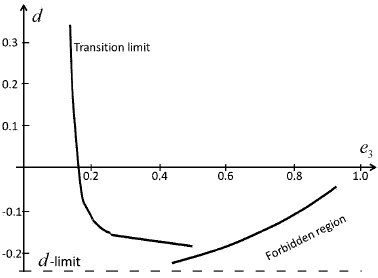
we come as before to continuous e3 -series for each d value and, furthermore, we again find limits. For d positive, and low e3 -values up to a definite limit, ω2 increases from pole to equator; thereafter, the tendency is inverted (Figure 1). For d negative (but greater than −1/4), another limit appears: as d becomes more and more negative, the e3 -series becomes shorter, because ω2 takes negative values, and the figures come into a forbidden region (Figure 1), a behavior that was also noticed in previous work.
5.2. The Heterogeneous Spheroidal Mass
The present series are more involved than those for the homogeneous case, so we must proceed care-fully and not try to get an overwhelming bulk of models that would render it difficult to give a clear panorama of their regularities. For this purpose, a basic series is constructed by fixing five parameters: ε= 1, e1 = 0.5, en = 0.1 and dn = da = −1/8, while the remaining one ea is let to vary in its allowed range.
5.2.1. The Case dn= da= −1/8
First, we take dn = da = −1/8 and allow ea to vary from 0.1 up to its maximum value, finding that equilibrium is possible for the angular velocity distribution given by equation (31) for the envelope and core. In Figure 2 we plot the angular velocity distribution in the nucleus (R < 0.5), and the atmosphere (R < 1); Figure 3 is a sketch of the model geometry.
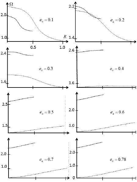
Fig. 2 Angular velocity distribution between pole (R = 0) and equator for the nucleus (shorter line) and atmosphere as ea varies from 0.1 (contact figure) to the limiting value 0.78. Fixed parameters are: e1 = 0.5, en = 0.1, dn = da = −1/8, ε = 1.
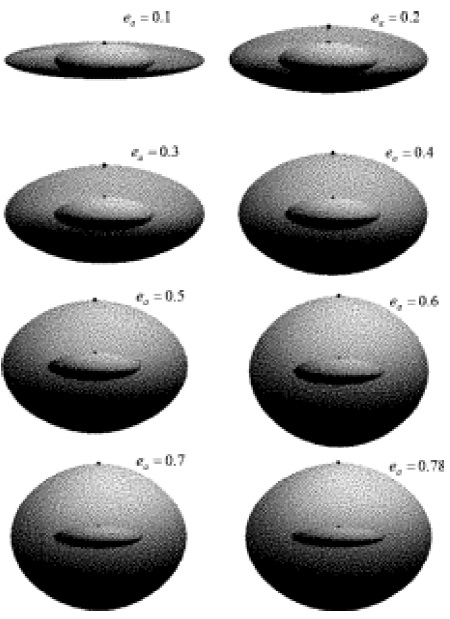
Fig. 3 Heterogeneous equilibrium figures as ea varies from 0.1 (contact figure) to the limiting value 0.78. Poles are suggested by a thick dot. Fixed parameters are: e1 = 0.5, en = 0.1, da = dn = −1/8, ε = 1.
In Figure 2 (see also Figure 3), the series begins with a contact figure in which the
poles of core and envelope touch each other, but not the equators, since the
equator of the atmosphere is twice as large as that of the nucleus
(e1 = 0.5). We see that the core rotates
slower than its envelope, even at the pole. In both, the angular velocity
decreases from pole to equator, i. e., the central parts rotate faster than
the outer ones. As ea increases (the atmosphere
expands),
5.2.2. The Case dn = da = 1/8
Here we take dn = da = 1/8 and let ea vary from 0.1 (contact figure) up. Once more, we get a set of series somewhat different from the former one (Figure 2), but also sharing several properties:
The series begins with a contact figure with the atmosphere rotating faster than the nucleus, as formerly.
Both differential angular velocities always monotonically decrease from pole to equator. In other words, there are not transition figures.
The limiting figure occurs at ea = 0.967 (zMa = 0.917).
The contact figure has a limit for en = 0.398 (cf. § 2.1.1).
The series do not end at en = 0.398; they continue for larger en and are more and more narrow, ending with an isolated figure with en = 0.4827, ea = 0.969 (zMn = 0.457) (see Figure 4).
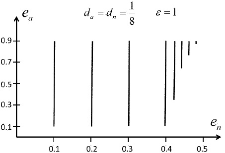
Fig. 4 Sketch of en -series for da = dn = 1/8, ε = 1. The series begin with a contact figure for en < 0.3975 and end at an ea around 0.9. After en = 0.3975 they become narrower and begin without a contact figure.
Hence, the plus sign of da, dn hinders the monotonous property of the angular velocity, and raises the upper limit of ea. Additionally, the series does not disappear after a last contact figure, but at a higher en limit.
5.2.3. The Case dn= 1/8, da= −1/8
This time, only dn sign is modified, so that our set of parameters is
Once more, the series starts with the contact figure ea = 0.0876; ea is established by zMa = zMn condition (equation (51)). The series resembles more the da = dn = −1/8 case than the da = dn = 1/8 one, in the sense that it has angular velocity transition limits and a limiting contact figure at en ≈ 0.4 (zMn = 0.38). For greater en values, there are, however, more series without an initial contact figure, which become narrower as en → 0.5 (zMn = 0.47). For en = 0.5 there only exists a series with the member ea = 0.97 (zMa = 0.92).
5.2.4. The Case dn = −1/8, da = 1/8
Here, da alone is modified relative to first case, so that the parameters values are now
With these parameters, we also establish series starting with a contact figure, when en < 0.4 (zMn = 0.43). Series without a contact figure are possible when 0.4 < en < 0.421; for en = 0.421 (zMn = 0.46) the series has a unique member at ea = 0.97. The atmosphere does not present angular velocity transition limits, and the nucleus has only one, at en = 0.2, ea = 0.6.
5.3. Consequences of the ε-value
To study the ε impact on our series, we assumed values for the parameters according to
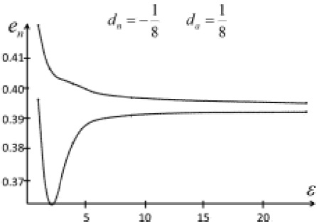
and constructed the series changing ea for a given en of a set 0.1 . . . 0.5, as formerly done. As an illustration, only cases dn = ∓1/8, da = ±1/8 were considered, and cases with dn = da = −1/8, 1/8 were disregarded. We refer briefly to these d-values as −+, +−, −−, and ++ (first sign for dn, second for da). Generally speaking, we did not find any new property, (other than those recognized above) when ε was modified, i. e., for each ε, the set of series can or cannot show angular velocity distribution ‘turning points’ (transition to monotonically increasing distribution), there is a final series having a contact figure, and there is a last (one-member) series. Clearly, as ε changes, the values characterizing a last contact figure, a last series, and a transition figure, must suffer modifications. The contact limiting figure has an en -value that first decreases and then increases, as ε increases from 1 to 24 (see Figure 5). On the other hand, en in the last series continually decreases as ε increases. The en span between last contact figure series and last series initially increases and thereafter continuously decreases (Figure 5).
5.4. Consequences of the e 1 -value
To study changes of our basic series (Figure 2) regarding the nucleus and atmosphere relative size e1, we varied it in steps of 0.1 from 0.9 down. We fixed da = ±1/8, dn = ±1/8, ε = 1 and constructed en series varying ea for each e1 value of the set. For example, when e1 = 0.9 we built the series for en = 0.1, 0.2, . . . . Qualitatively again, we found series with or without transition limits, ea upper limits, last contact figure for en series, and final one-member series. Quantitatively, there are differences regarding the above results. The ω2 magnitudes and the variation range change; the en gap between last contact figure and last one-member series grows as e1 decreases, starting at e1 = 0.5; likewise, beyond e1 = 0.5 the gap approaches 0 (see Figures 6 and 7). This behavior is somewhat similar to the ε-effect (Figures 4 and 5): as e1 or ε increases the gap be-comes narrower, and finally it disappears.
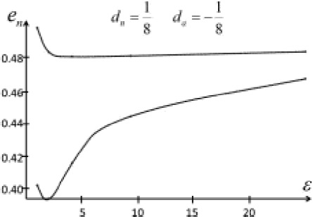
Fig. 6 As ε increases, the last contact figure en (lower curve) first decreases and then increases slowly; on the contrary, last one-member series en decreases continually. Both curves tend to the same point, i. e., last contact figure is at the same time last one-member series.
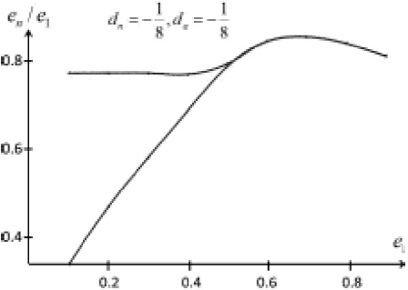
Fig. 7 As e 1 increases, the last contact figure en /e1 (lower curve) increases continuously, practically for all e1 values; on the contrary, for the last one-member series en /e1 remains constant up to about e1 = 0.5. Both curves coincide after about e1 = 0.5. The curves were plotted for dn , da = −1/8.
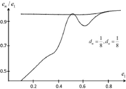
Fig. 8 As e1 increases, the last contact figure en /e1 (lower curve) increases continuously with some small oscillation, for all e1 values; on the contrary, the last one-member series en /e1 remains constant (≈ 0.98) practically all the way. Both curves coincide after about e1 = 0.7. The curves were plotted for dn , da = 1/8

