


 nova página do texto(beta)
 Inglês (pdf)
 Artigo em XML
 Referências do artigo
 Enviar este artigo por email
 Citado por SciELO
  Similares em
SciELO
Similares em
SciELO 
 Permalink
1. Introduction
Even though it is clear that the Herbig-Haro objects HH 1 and 2 have strong time-variabilites (Herbig 1969, 1973; Herbig & Jones 1981; Brugel et al. 1985; Raga et al. 1990a; Böhm et al. 1993; Eislöffel et al. 1994), the study of their time-dependent emission spectrum has proven to be quite difficult. The difficulties arise from the heterogeneity of the data.
The older images of HH 1 and 2 (before ≈ 1985) are relatively broad band photographic plates, and have been analyzed by Herbig (1969, 1973) for time variabilities. The analysis presented in these papers to some extent stands alone, since it is not straight-forward to relate it to more recent observations (obtained with different techniques).
More recent CCD images of HH 1 and 2 obtained through narrow-band filters, cover very few emission lines, and in general lack any calibration. As far as we are aware, the only attempts to use ground based CCD images for an evaluation of the variability of HH 1 and 2 were presented by Raga et al. (1990a) and by Eislöffel et al. (1993).
Spectrophotometric observations of HH 1 and 2 have generally been obtained either with “short” (Hartigan et al. 1987) or “long” (Solf et al. 1988; Giannini et al. 2015) spectrograph slits. Though the obtained spectra are generally well calibrated, it is difficult to disentangle the time-variability of the angularly extended HH 1 and 2 objects from effects due to different slit sizes and positions of the successive observations. Also, spectrophotometric observations of Brugel et al. (1981a, b) are available, which cover at least most of the emitting regions of HH 1 and 2 (see below and § 2).
The HH 1 and 2 images obtained with the Hubble Space Telescope (Hester et al. 1998; Bally et al. 2002; Hartigan et al. 2011; Raga et al. 2015a, b; Raga et al. 2016) have calibrated fluxes, and are therefore appropriate for studying the time-dependence of the emission. An analysis of the time-variability of the [O III] 5007, Hα and [S II] 6716+30 emission of HH 1 in this images was presented by Raga et al. (2016). Also, a “pre-COSTAR” set of HST images of HH 2 (in Hα, [S II] and [O III]) was obtained by Schwartz et al. (1993).
In Figure 1 we present a comparison between a photograph of HH 2 obtained by Herbig in 1959 (in red light, with the Lick Observatory 120-inch reflector shortly after its inauguration), and the addition of an Hα and a [S II] 6716+30 frame obtained with the Hubble Space Telescope in 2014 (see Raga et al. 2015a, b). The two images have been scaled and centered in an approximate way. From this figure, it is clear that the structure of HH 2 has changed in a dramatic way over the past ≈ 55 years.
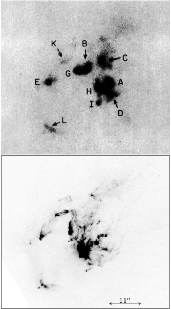
Fig. 1 Comparison between a photograph of HH 2 (obtained by G. Herbig in 1959 at the Lick Observatory 120-inch reflector, top) and an Hα+[S II] image (obtained in 2014 with the HST, shown with a linear greyscale). The two images have been approximately scaled and centered relative to each other. The identifications of the condensations of HH 2 are given in the top frame, and the angular scale is shown in the bottom frame. N is up and E to the left.
In the present paper, we use the two sets of HST images which cover a broader range of emission lines, namely,
the 1994 images of Hester et al. (1998), which include filters isolating the [O III] 5007, Hα and [S II] 6716+30 lines,
the 2014 observations of Raga et al. (2015a, b) which include the Mg II 2798 (not described in the published papers), [O II] 3726+28, Hβ, [O III] 5007, [O I] 6300, Hα and [S II] 6716+30 lines.
The second (2014) set of HST images covers most of the bright near-UV to optical emission lines of HH 1 and 2, and is therefore appropriate for studying the time-evolution of the spectra of these objects. Unfortunately, the first (1994) set has only three images, and can only be used for an analysis of the time-evolution of the three line combinations.
For an analysis of more emission lines, we can use the spectrophotometric observations of Brugel et al. (1981a). These authors used a multi-channel spectrophotometer with apertures that covered most of the emitting regions of HH 1 and 2. These observations can be directly compared with line fluxes calculated by angularly integrating the 1994 and 2014 sets of HST images over the emitting areas of HH 1 and HH 2.
In this way, we use the immensely detailed HST images only for obtaining an angularly integrated emission line spectrum of HH 1 and 2, and we compare the resulting spectra with the spectrophotometric observations of Brugel et al. (1981a). We feel that the somewhat brutal angular integration of the HST images is justified by the very interesting comparison that can be made with the older spectrophotometric results.
The paper is organized as follows. The HST images and the older, spectrophotometric data sets are discussed in § 2. The 2014 Mg II 2798 HST image (which has not been presented before in the literature) is also presented in this section. § 3 presents an evaluation of the time-evolution of the emission line spectra of HH 1 and 2. § 4 discusses a simple working surface model which is used for interpreting the observed time-dependence of the line emission. Finally, the results are discussed in § 6.
2. The observations
2.1. The reddening correction
Brugel et al. (1981a) used Miller’s (1968) method, which is based on the fixed ratio of the transauroral (4069, 4076Å) to the auroral (10318, 10336 Å) [S II] lines, and obtained E(B − V) = 0.47 for HH 1 and E(B −V) = 0.35 for HH 2. Raga et al. (2015b) used the average of the Hα/Hβ ratios of the individual emitting pixels of HH 1 and 2 to derive E(B − V) ≈ 0.27 for the two objects.
In this paper, we present the observed line fluxes and ratios, as well as the values corrected for a standard Galactic extinction curve with E(B − V) = 0.27. This extinction curve (see Fitzpatrick 1999) corresponds to the R = A V /E(B − V) = 3.1 case of Cardelli et al. (1988). This choice is not unique, since there has been a considerable amount of discussion as to which extinction curve is actually relevant for the HH 1/2 region (see, e.g., Böhm-Vitense et al. 1982 and Böhm et al. 1991). The choice of extinction curve of course has a particularly strong effect in the UV.
2.2. The first epoch spectrophotometric observations
In September 1978, Brugel et al. (1981a) observed HH 1 and 2 with the MCSP II spectrophotometer (see Oke 1969) at the Palomar 5.1 m telescope. In the configuration that was used the spectrophotometer had an aperture of 6′′ diameter (see Brugel et al. 1981b), and several positions (2 for HH 1 and 3 for HH 2) were used to cover the emitting regions of HH 1 and 2. We have now co-added the spectra from the two HH 1 apertures and the three HH 2 apertures to obtain two spectra: one for HH 1 and one for HH 2.
These spectra include the [O II] 3726+28, Hβ, [O III] 5007, [O I] 6300 and Hα lines. Unfortunately, the channels of the MCSP cover the [S II] 6716 but not the [S II] 6730 line. Because of this, we have taken the [S II] 6716+6730/Hα ratio from a lower quality spectrum obtained by Brugel et al. (1981a) at the KPNO 2.1 m telescope.
Finally, for the Mg II 2798 line we have taken the fluxes obtained in 1980 with the International Ultraviolet Explorer (IUE) by Böhm-Vitense et al. (1982). The IUE spectrograph had a 23′′ ×10′′ aperture, which included most of the emitting regions of HH 1 and 2. As this UV observation was carried out only a couple of years after the Brugel et al. (1981a) optical observations. In the following we consider them as taken at the same time.
2.3. The HST images
We consider two epochs of HST images:
the [S II] 6716+30, Hα and [O III] 5007 images of Hester et al. (1998), obtained in 1994.6,
the [S II] 6716+30, Hα, [O I] 6300, [O III] 5007, Hβ, and [O II] 3726+28 images of Raga et al. (2015a), obtained in 2014.6.
To the 2014.6 set of images, we have added a Mg II 2798 image (a 5484 s exposure through the F280N filter) which was not analyzed by Raga et al. (2015a). Figure 2 shows the brighter region of HH 2 in the Hα, Hβ, and Mg II 2798 dereddened images, and the Mg II/Hβ line ratio map. HH 1 is barely visible in the Mg II 2798 frame, but an angularly integrated flux for HH 1 can be obtained.
There are two other epochs of HST images of HH 1 and 2 (see Bally et al. 2002 and Hartigan et al. 2011), but we do not include them in the present study because they only cover the [S II] 6716+30 and Hα lines.
As discussed by Raga et al. (2015a), the continuum emission of HH 1 and 2 affects the line fluxes obtained from the HST images. This continuum contamination is more important for the blue lines, and it could be as large as ≈ 30% for the Mg II 2798 line. However, this is unlikely to have a large effect for the qualitative interpretation of the emission proposed in the present paper.
In order to compare the HST line fluxes with the spectrophotometric data of Brugel et al. (1981a), we carry out angular integrations over the emitting areas of HH 1 and 2 in the HST frames. In order to do this, we add the emission within the 5 × 10⁻¹⁵ erg s−1cm−2arcsec−2 (dereddened) Hα isophotes of HH 1 and 2. In this way, we avoid defining arbitrary “boxes” around both objects.
2.4. The Mg II 2798 image
Figure 2 shows the Mg II 2798 HST image obtained in 2014 (see subsection 2.3). We see that the Mg II emission has an angular extent comparable to that of the Hβ emission (fainter, more extended regions being seen in Hα). Because of this, we have chosen to calculate the Mg II/Hβ ratio map (which depends much less on the reddening correction than the Mg II/Hα ratio), which is also shown in Figure 2. We do not display the Mg II emission of HH 1 be-cause it is quite faint, so that it is only appropriate for obtaining an angularly integrated line flux.
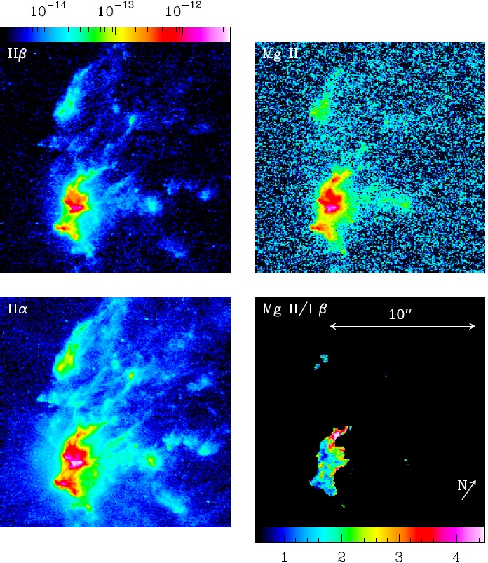
Fig. 2 Hβ (top left), Hα (bottom left), Mg II 2798 (top right) and Mg II/Hβ line ratio (bottom right) maps of HH 2. The emission maps are shown with the logarithmic color scale (in erg s−1 cm−2 arcsec−2) displayed in the top left bar. The line ratio map is shown with the linear color scale displayed in the bottom right bar. The angular scale and orientation of the frames are shown in the bottom right frame. The color figure can be viewed online.
From the line ratio map, we see that most of the Mg II emitting region of HH 2 (within condensation H) has a Mg II/Hβ ratio of ≈ 1 → 2. If one looks at the predictions from the plane-parallel shock models of Hartigan et al. (1987), one sees that these line ratios are consistent with shock velocities between 110 and 160 km s−1.
There is also a small region in the NE of condensation H with Mg II/Hβ ≈ 5, implying a shock velocity of ≈ 260 km s−1 (see Hartigan et al. 1987).
3. The time-dependent line ratios and fluxes
In Table 1, we present the observed and dereddened Hα fluxes obtained in the three epochs of observations described in § 2. This table gives the measured (F) as well as the dereddened (F0) fluxes, which were obtained assuming a standard Galactic extinction curve with E(B − V) = 0.27 (for both HH 1 and 2, see § 2.1). We have also computed the Hα luminosities with the dereddened fluxes and a distance of 414 pc to HH 1 and 2.
Table 1 Hα line fluxes and luminosities.
| Epoch | HH 1 | HH 2 | ||||
|---|---|---|---|---|---|---|
| FH α1 | FH α,01 | LH α2 | FH α1 | FH α,01 | LH α2 | |
| 2014.6 | 4.16 | 7.50 | 4.05 × 10⁻³ | 33.67 | 60.75 | 3.28 × 10⁻² |
| 1994.6 | 5.50 | 9.92 | 5.36 × 10⁻³ | 19.21 | 34.67 | 1.87 × 10⁻² |
| 1978.7 | 5.77 | 10.41 | 5.63 × 10⁻³ | 7.88 | 14.21 | 7.68 × 10⁻³ |
1Observed (F) and dereddened (F0) Hα fluxes in units of 10−13 erg s−1 cm−2.
2Luminosities (in units of L⊙) assuming a distance of 414 pc.
It is clear that the Hα luminosity of HH 1 has a slowly decreasing trend, with a decrease of ≈ 4% from 1978.7 to 1994.6 and a somewhat larger decrease of ≈ 24% from 1994.6 to 2014.6. On the other hand, HH 2 has an Hα luminosity which increases by a factor of ≈ 2.4 from 1978.7 to 1994.6 and by a factor of ≈ 1.75 from 1994.6 to 2014.6.
In Table 2, we present the observed and dereddened line ratios of HH 1 and 2. For both objects, the spectrum has a surprisingly small time-dependence. For HH 1:
the Mg II 2798 line (relative to Hα) has not changed appreciably from 1980.7 to 2014.6. Unless we have a strange coincidence, this result seems to imply both that the variations of the intrinsic spectrum are small and that the extinction to HH 1 has remained invariant during this time-period,
the [O II] 3726+29 lines have grown by ≈ 40% from 1978.7 to 2014.6,
the Hβ line has a relatively low value compared to Hα in the 1978.7 spectrum. This might be an indication that the regions of HH 1 with collisionally excited lines could have contributed more to the spectrum of HH 1 than in 2014.6 (when the regions of high Hα/Hβ ratio have small angular extents, see Raga et al. 2015b),
the [O III] 5007 line grew by a factor of 2 from 1978.7 to 1994.6, and then decreased by ≈ 20% in the 2014.6 observations,
the [O I] 6300 line has had a small increase from 1978.7 to 2014.6,
the [S II] 6716+30 lines have grown (relative to Hα) by a factor of ≈ 2 from 1978.7 to 2014.6.
Table 2 Emission lines with respect to Hα = 100
| Ion | λ [Å] | Epoch | HH 1 | HH 2 | ||
|---|---|---|---|---|---|---|
| F | F0 | F | F0 | |||
| Mg II | 2798 | 2014.6 | 10 | 39 | 16 | 60 |
| 1980.7 | 8 | 33 | 8 | 31 | ||
| [O II] | 3726+29 | 2014.6 | 54 | 115 | 36 | 76 |
| 1978.7 | 31 | 66 | 27 | 58 | ||
| Hβ | 4861 | 2014.6 | 26 | 35 | 24 | 33 |
| 1978.7 | 17 | 23 | 22 | 30 | ||
| [O III] | 5007 | 2014.6 | 14 | 19 | 16 | 21 |
| 1994.6 | 18 | 23 | 21 | 28 | ||
| 1978.7 | 9 | 12 | 15 | 20 | ||
| [O I] | 6300 | 2014.6 | 40 | 42 | 43 | 45 |
| 1978.7 | 34 | 36 | 41 | 43 | ||
| Hα | 6563 | 100 | 100 | 100 | 100 | |
| [S II] | 6716+30 | 2014.6 | 87 | 85 | 46 | 45 |
| 1994.6 | 68 | 66 | 40 | 41 | ||
| 1978.7 | 49 | 48 | 38 | 37 | ||
For HH 2:
the Mg II 2798 line has grown by a factor of 2 from 1980.7 to 2014.6. This could be due to the fact that the aperture of the IUE spectrograph (used for the 1980.7 observations see § 2) might not have included all of the emitting region of HH 2. Also, the continuum contamination in the HST image could be responsible for part of this increased flux (however, a corresponding in-crease should then be seen in HH 1),
the [O II] 3726+29 lines have grown (relative to Hα) by ≈ 20% from 1978.7 to 2014.6,
the [O III] 5007 line grows by ≈ 40% from 1978.7 to 1994.6, and in 2014.6 returns to a value very similar to the 1978.7 value,
the Hβ, [O I] 6300 and [S II] 6716+30 lines have very small variations (relative to Hα).
4.Interpretation in terms of a working surface model
4.1. General considerations
The variations in the emission line ratios for HH 1 are not large, but might be significant (in particular, for the [S II] and [O II] lines). The spectrum of HH 2 shows smaller line ratio variations, except for the Mg II 2798 line (an effect which might be due to part of the emitting region falling outside the IUE spectrograph aperture of the 1980.7 observations). Therefore, we conclude that the emission line spectra of HH 1 and 2 have at most shown small variabilities in their relative line intensities (see Table 2).
HH 1 shows a small decrease in Hα flux of ≈ 30% from 1978 to 2014. On the other hand, the Hα flux of HH 2 shows a clear, monotonic increase as a function of time.
Unless we have a combination of effects cancelling each other out, we can conclude that the invariance of the line ratios implies that:
a time-independent interstellar extinction correction (such as the one which we have applied, see § 2) appears to be appropriate,
the shock velocities associated with HH 1 and 2 do not change substantially as a function of time.
As can be seen from steady, plane-parallel shock models (see, e.g., Raymond 1979 and Hartigan et al. 1987), the emission line ratios of the spectrum emitted by a shock are generally a strong function of shock velocity, and only depend weakly on the pre-shock density. Also, shocks (of a given shock velocity) with a cooling function dominated by processes in the “low density regime” have line fluxes that scale linearly with the preshock density.
Therefore, an increase in the emission line flux (and at the same time keeping approximately constant line ratios) such as is seen in HH 2 implies that the emission is produced in shocks with approximately time-independent shock velocities, and with a pre-shock density that increases with time. How can this situation be obtained in a working surface of a jet? This question is addressed in the following section.
4.2. The luminosity of a working surface
A working surface is composed of a “jet shock” that slows down the jet material (on interaction with the environmental gas) and a “bow shock” which accelerates ambient material. From the standard, ram-pressure balance argument, for the two-shock working surface one obtains a velocity of motion (Raga et al. 1990b):
where vj is the jet velocity,
The jet shock has a shock velocity:
And the shock velocity of the bow shock is:
Now, in a highly radiative shock most of the kinetic energy flux arriving at the shock ends up being radiated away. Therefore, assuming that the jet and bow shocks have approximately the same surface area σ, the luminosities of the jet shock and the bow shock are:
where we have used equations (1-3) to write the shock luminosities in terms of the jet velocity vj (second set of equalities) and in terms of the working surface velocity vws (third set of equalities). In these equations, Mj = σρj vj is the total mass per unit time arriving at the working surface.
The total luminosity of the working surface then is:
As discussed in the previous section, the fact that the emission line ratios of HH 1 and 2
have changed very little implies that the shocks giving rise to the observed
emission have relatively constant shock velocities. Unless one is prepared to
believe in the presence of a calibrated balancing of different effects, the fact
that we have constant jet shock or bow shock velocities (depending on which of
the two shocks dominates the emission) implies constant values of
4.3. Application of the working surface model to HH 1 and 2
The emission line spectrum of HH 2, which shows basically time-independent line ratios (indicating a constant shock velocity) and a strongly increasing luminosity can then be directly interpreted as a jet (of constant velocity and mass loss rate) travelling in an environment of increasing density. From equation (7) we see that the increase in the environmental density is expected to be proportional to the observed increase in the luminosity.
For HH 1, we observe a small decrease in luminosity as a function of time (see Tables 1 and 2). In terms of our working surface model, this would then imply that HH 1 is moving into an ambient medium of slowly decreasing density (see equation 7).
Let us note that a “high β”, “heavy jet” situation is consistent with the high proper motions observed in HH 1 and 2. These proper motions have remained almost constant from the mid-twentieth century (see Herbig & Jones 1981; Bally et al. 2002), implying that the presence of environmental inhomogeneities do not produce appreciable effects (as would be the case for a low β outflow, see equation 1). Interestingly, a small acceleration of the HH 1 proper motions has recently been measured (Raga et al. 2016), which would be consistent with a high β jet moving into a medium of decreasing density (see equation 1).
Implicit in this discussion is the expectation of a time-independent ratio between the luminosity of the lines we are studying (see Tables 1 and 2) and the continuum and line luminosities (at optical, UV and IR wavelengths) not considered in the present study. This appears to be a reasonable assumption given the fact that we are apparently having almost time-independent shock velocities in HH 1 and 2.
4.4. The mass loss rate of the HH 1/2 system
From Table 2, we see that the ratio of the luminosities of all of the lines (including Hα) we are considering to Hα lies in the range of 3 to 4 for HH 1 and 2. In the 1978.7 observations of Brugel et al. (1981a), one finds that the remaining lines (observed by these authors, but not included in our present paper) contribute an extra ≈ 30% to the luminosities of HH 1 and 2. The continuum of HH 1 and 2 has a luminosity of ≈ 2 times the Hα luminosity in the λ = 3000 to 8000 Å wavelength range (Brugel et al. 1981b).
The continuum in the λ = 1300 to 3000 Å wave-length range (Böhm-Vitense et al. 1982) has a luminosity of ≈ 15 times Hα. However, the reddening correction in the far UV is very uncertain (Böhm et al. 1991).
Considering the line and continuum contributions described above, we see that the total luminosity of HH 1 and 2 is at least ≈ 10 times the Hα luminosity. Therefore, in the first (1978.7) epoch, both HH 1 and HH 2 had total luminosities of ≈ 7 × 10⁻² L⊙ (see Table 1). Inserting this value in equation (7), we then obtain an estimate:
where we have used an estimate of 200 km s−1 for the velocity of HH 1 and 2 (see, e.g., Bally et al. 2002).
Since HH 1 and 2 appear to correspond to high
5. Conclusions
A comparison of spectra of HH 1/2 obtained in three epochs, namely
1978.7: spectrophotometric data of Brugel et al. (1981a),
1994.6: 3 narrow-band HST images (Hester et al. 1998),
2014.6: 7 narrow-band HST images (Raga et al. 2015a, b),
shows that the emission-line ratios do not change appreciably over this rather extended time period. This result is not completely surprising because the proper motion velocities of these objects have remained almost constant over a long time period (see Herbig & Jones 1981 and Bally et al. 2002).
More surprising is the fact that while the line intensities of HH 1 have remained almost constant (showing only a small decrease of ≈ 30% in the 1978-2014 period), HH 2 has brightened by a remarkably large factor of ≈ 4. This scaling up of the brightness of HH 2 is unlikely to be the result of a change in the extinction to the object (as it travels away from the outflow source), because such a change would be directly visible as a time-dependence of the observed line ratios.
Therefore, we conclude that HH 2 appears to be moving into an ambient medium of increasing
densities, while preserving the same shock velocity. This situation is consistent
with the leading working surface of a “heavy” jet (i.e., with high
A simple analytic model of a working surface shows that for a high β working surface the luminosity is proportional to ρa /ρj. Therefore, the increase of ≈ 4 in the brightness of HH 2 could be explained with a similar rise in the density of the environment into which HH 2 is travelling.
Of course, in this high β regime the changes in environmental density will also lead to (small) changes in the motion of the HH objects. The small decrease in the brightness of HH 1 (interpreted as the result of a decrease in the environmental density) would then be coupled with a small increase in the velocity of the object. It seems that such an effect is indeed observed (Raga et al. 2016).
Clearly, it will be necessary to carry out a new analysis of the proper motions of HH 2 (including the new HST images of Raga et al. 2015a, b) to see whether or not its increase in brightness is coupled with a small decrease in its proper motion velocities.
Another remaining point is that it is clear that the total (radiative) luminosity of an HH object provides a direct measure of the mechanical luminosity of the associated stellar outflow (see § 4.2). In § 4.4, we have used an estimate of the luminosities of HH 1 and 2 to obtain an estimate of the mass loss rate associated with this outflow. The luminosity that we have used is based on the optical line intensities (which have been measured at different epochs), the optical continuum (obtained only around 1980), and the line and continuum UV emission (also obtained around 1980). Notably, we did not include the IR line and continuum emission (part ot this information is present in Spitzer and Herschel observations of the HH 1/2 region, see Noriega-Crespo & Raga 2012 and Fischer et al. 2010). A detailed analysis of current observations covering all of the relevant wavelength ranges would provide more reliable luminosities for HH 1 and 2, therefore leading to better estimates of the mass loss rate of the outflow.

