


 nova página do texto(beta)
 Inglês (pdf)
 Artigo em XML
 Referências do artigo
 Enviar este artigo por email
 Citado por SciELO
  Similares em
SciELO
Similares em
SciELO 
 Permalink
1. Introduction
Low-mass young stellar objects (YSOs) are newly born stars that are not yet burning hydrogen
in their cores. Most of them are embedded in their parental molecular clouds and
are, therefore, obscured at optical wavelengths. At radio wavelengths
The present paper is the first in a new series reporting on radio observations of additional nearby regions of star formation
1.1. Barnard 59 and Lupus 1
The Pipe Nebula is a large molecular complex composed of several dark clouds (Barnard 1919: Lynds 1962). Among those, B59 stand out as the only one with significant star formation activity (Alves, Lombardi & Lada 2008). There are 20 catalogued young stars in B59 in an area of 15' x 15', of which 15 are T Tauri star candidates (Brooke et al. 2007). Recently, Dzib et al. (2013b) presented radio observations that covered the central region of B59 and detected five radio sources associated with five of the YSOs reported from the Spitzer observations of Brooke et al. (2007). These are thought to be thermal radio sources because of their SED classification and the Lbol -Lradio ratio, which agrees well with that expected from the correlation of free-free radio continuum and the stellar luminosity (e.g., AMI Consortium et al. 2011). The observations presented here expand upon those reported by Dzib et al. (2013b) and include the 20 YSOs reported by Brooke et al. (2007).
In his recent review, Comerón (2008) recognized Lupus as one of the main low-mass star-forming-region complexes within 200 pc of the Sun. The complex is divided into nine individual clouds, labeled as Lupus 1 to 9 (i.e., Hara et al. 1999), and they extend down to declinations as low as -44°. The present study is restricted to the higher declination cloud (Lupus 1) at -35°. Lupus 1 was the first cloud in the Lupus region where T Tauri stars were discovered (Henize 1954). Nowadays, up to 13 classical T Tauri stars are known to be present in Lupus 1 (Comerón 2008), and some additional candidates have been suggested by Merin et al. (2008) using the Spitzer Space Telescope. These YSOs are sparsely distributed suggesting that an isolated mode of star formation is at work. The observations presented here will cover the 13 known T Tauri stars in Lupus 1.
2. Observations and source selection
The observations were collected on 2014 March 6 (Lupus 1) and 20 (B59) with the VLA of the National Radio Astronomy Observatory (NRAO1) in its most extended (A) configuration. The C band receiver was used and four frequency sub-bands, each 1 GHz wide and centered at 4.5, 5.5, 6.5, and 7.5 GHz, respectively, were recorded simultaneously with 3-bit sampling. For each region, nine target fields were observed. The fields in B59 were distributed around the core in a semi-mosaic configuration (Figure 1; left panel), while those in Lupus 1 were distributed so as to observe known YSOs (Figure 1; right panel). The phase calibrators were J1700-2610 and J1607-3331 for B59, and Lupus 1, respectively.
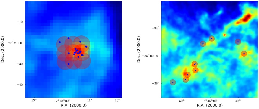
Fig 1 Mapped areas in B59 (left) and Lupus 1 (right). The red circles indicate the observed VLA fields. The diameter of each circle is 8' in B59 and 12/5 in Lupus 1 (see text). Blue dots are known YSOs. Background: IRAS images at 100 μm of the B59 and Lupus 1 region (Neugebauer et al. 1984). The color figure can be viewed online.
The total observing time per epoch was one hour. At the beginning of the observations, the first 10 minutes were spent on the flux calibrator 1331+305=3C286; part of this scan was spent slewing the antennas and setting up the correlator. Subsequently, the phase calibrator was observed for five minutes (again part of this time was spent slewing the antennas). Finally, a cycle with three succesive target scans (each 4.5 minutes long) and one phase calibrator scan (1 minute) was repeated until all the targets were observed.
The data were edited and calibrated using the Common Astronomy Software Applications (CASA v4.2.2) package, with the VLA calibration pipeline vl.3.1. The bootstrapped flux density at vcentral = 6.0 GHz for the phase calibrator J1700-2610 was 1.96 ±0.02 Jy, with a spectral slope α = 0.10. For J1607-3331, the bootstrapped flux density (also at 6 GHz) was 0.168 ±0.002 Jy, with α = -0.41.
To obtain the highest sensitivity for the target fields, the four sub-bands were jointly imaged using a multi-frequency deconvolution (e.g., Rau & Cornwell 2011). Additionally, in B59 we combined the fields in mosaic mode (imagermode='mosaic' in CASA) to gain further sensitivity. The pixel size was set to 0'.'06, and a weighting scheme intermediate between natural and uniform was used (robust=0.0 in CASA). Also, the minimum level of the primary beam was set and corrected at a response of 20% (PBCOR=True and MINPB=0.2 in CASA). The resulting mosaic in B59 covered an area of 316 arcmin2. In the case of Lupus 1, each field covered a circular with a diameter of 12/5. The parameters of the maps are given in Table 1.
Table 1 Observations and final parameters of maps.
| Region | Date | Synthesized beam | rms noise |
|---|---|---|---|
| (dd.mm.yy) | (θmaj X θmin ; P.A.) | (μJy brn -1 ) | |
| B59 | 20.03.14 | 0''.78x0''26; 28.8° | 9 |
| Lupus 1 | 06.03.14 | 0''87x0''24; 4.9° | 15 |
A visual inspection of the images was first performed at the position of known YSOs to look for detections. We considered a radio source to be the counterpart of a YSO when it had a flux density larger than four times the noise level in the images, and coincided with the position of a previously reported YSO to within 1". This corresponds to our angular resolution. Furthermore, an automated search for additional radio sources present in the mapped areas was performed using a specialized software, as we now describe.
An important element in the process of source extraction is to have the correct noise map. The rms estimation algorithm of the sExtractor package (Bertin & Arnouts 1996) was used to create a suitable noise map. This algorithm defines the rms value for each pixel in an image by determining the distribution of pixel values within a surrounding local mesh until all values are around ±3 × σrms. This method ensures that most of the real emission is removed from the noise image and the determined noise map contains the correct noise level. Once the rms map has been constructed, the source extraction was done using the BLOBCAT package (Hales et al. 2012). This software is written in the scripting language Python and utilizes the flood fill algorithm to detect and catalog blob sources in two dimensional astronomical images. It separates individual blobs from a dimensionless signal-to-noise (SNR) map. The SNR map is the result of a ratio between the input image and the given rms map. The extraction was performed, in the SNR map, searching all pixels and their neighbors, with a 5 × σrms threshold. In this case, only the sources with integrated fluxes and peak fluxes above 5 × σnoise were considered to be real. This allows us to weed out noise peaks from real sources.
It is worth to briefly explain why a threshold of 4σ was chosen for radio sources associated with known YSOs, whereas 5σ was required for sources with no known counterparts. As explained in detail in Pech et al. (2016), in an image where the noise level is σ and where no sources at all are present, there is a probability of 2.87×l0-7 that any given independent pixel will have emission at 5σ or more. We emphasize that the presence of such a 5σ peak is entirely due to random noise fluctuations, and not to a real source. As mentioned earlier, the area of our B59 mosaic is 316 arcmin2, and our resolution element (0"78 × 0"26) has an area of 5.63 × l0-5 arcmin2. Thus, there are 5.6 × l06 independent resolution elements in our mosaic, and we expect at most (5.6 × l06) × (2.87 × l0~7) = 1.6 noise peaks at 5σ or more in our image. Thus, most of the sources detected at more than 5σ must be real sources rather than noise peaks. We note that if we had chosen 4σ instead, the expected number of false-positive detections would have increased to the completely unacceptable figure of 178. In the case of our search around known YSOs, the search area is limited to 1 arcsec2 (see above), which corresponds to barely 5 resolution elements. The probability of encountering a 4σ peak in such a small area is extremely small (less than 0.02%), so any source detected at more than 4σ is very likely real.
3. Results
3.1. Radio Sources in B59
A total of 56 sources were detected in the B59 region, nine of them associated with known YSOs (their derived parameters are given in Table 2). Five of these sources were previosuly detected at radio wavelengths by Dzib et al. (2013b) while the other four are reported here for the first time. The remaining sources are most likely associated with extragalactic objects and are discussed below. The deconvolved sizes of most of the detected YSOs are consistent with a point source structure. The only exceptions are [BHB2007] 11 with a deconvolved size of 0".43±0".07×0".37±0".08 at PA=170°±46°, and [BHB2007] 10 with a deconvolved size of 0".50±0".25×0".24±0".06 at PA=35°±09°.
Table 2 Radio properties of YSOS in B59.
| YSO | SED | VLA Position | Sv ± σsva | α | |
|---|---|---|---|---|---|
| Name | Class | Ra | Dec. | (μJy) | |
| [BHB2007] 1 | Flat | 17hllm03.S937 ± 0.s003 | -27°22'55".26 ± 02.06 | 81 ± 19 | 1.9 ± 1.4 |
| [BHB2007] 2 | II | 17h11m04.s137 ± 0.s004 | -27°22'59".39 ± 0".09 | 80 ± 29 | 0.7 ± 1.4 |
| [BHB2007] 3 | II | 17h11m11.s826 ± 0.s003 | -27°26'55".10 ± 0".10 | 43 ± 18 | <0.2 ± 1.7 |
| [BHB2007] 4 | II | … | … | <36 | … |
| [BHB2007] 5 | II | … | … | <36 | … |
| [BHB2007] 6 | II | … | … | <36 | … |
| [BHB2007] 7 | Flat | 17h11m17.s286 ± 0.s003 | -27°25'08".36 ± 0".06 | 77 ± 20 | -4.0 ± 1.6 |
| [BHB2007] 8 | II | … | … | <36 | … |
| [BHB2007] 9 | Flat | 17h11m21.s553 ± 0.s002 | -27°27'42".17 ± '".04 | 73 ± 21 | 0.8 ± 1.0 |
| [BHB2007] 10 | I | 17h11m22.s161 ± 0.s003 | -27°26'02".02 ± 0".06 | 135 ± 24 | 0.7 ± 1.2 |
| [BHB2007] 11 | 0/I | 17h11m23.s118 ± 0.s001 | -27°24'32".56 ± 0".02 | 643 ± 30 | -0.1 ± 0.3 |
| [BHB2007] 12 | II | … | … | <36 | … |
| [BHB2007] 13 | II | 17h11m27.s017 ± 0.s002 | -27°23'48".68 ± 0".06 | 58 ± 14 | 1.0 ± 1.8 |
| [BHB2007] 14 | II | … | … | <36 | … |
| [BHB2007] 15 | II | … | … | <40 | … |
| [BHB2007] 16 | II | … | … | <40 | … |
| [BHB2007] 17 | II | … | … | <36 | … |
| [BHB2007] 18 | II | 17h11m41.s.8402 ± 0.s0005 | -27°25'47".72 ± 0".01 | 329 ± 18 | -0.0 ± 0.3 |
| [BHB2007] 19 | II | … | … | <36 | … |
| [BHB2007] 20 | II | … | … | <36 | … |
aAverage integrated flux density over the full 4.0-8.0 GHz bandwidth. Upper limits are at four times the noise level.
As a first attempt to determine the spectral index, α (defined as
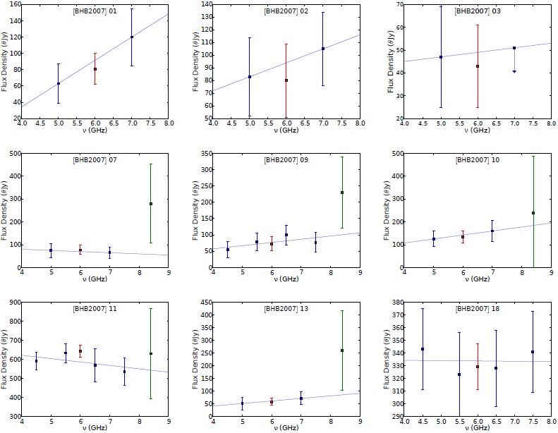
Fig. 2 Spectral index fitting for the sources detected in B59, using the images obtained in independent sub-bands (blue points). The red points at 6 GHz are the flux densities of four combined sub-bands. Green points are the fluxes measured by Dzib et al. (2013b) at 8.4 GHz, and their error bars are the result of adding in quadrature the flux errors as reported by Dzib et al. (2013b) and the uncertainties for the spectral index fitting. The color figure can be viewed online.
3.2. Radio Sources in Lupus 1
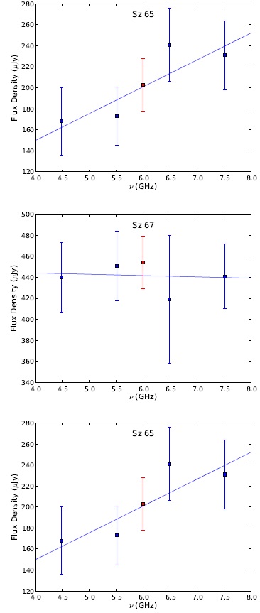
In the single fields corresponding to Lupus 1, a total of 58 sources were detected, four of them associated with known YSOs. This is the first time, to our knowledge that these sources are detected at radio wavelengths. The nature of the remaining sources is unclear, but most of them are likely associated with extragalactic objects, as we will discuss below. The radio properties of the detected YSOs are shown in Table 3. The deconvolved structure for all of them is consistent with their being point sources. Similarly to what was done for B59, the data were split in order to determine the spectral index of the detected YSOs. The resulting spectral indices are given in Table 3 and the fits are shown in Figure 3. All the YSOs detected in Lupus 1 are close to the phase center of their observations, so the beam squint effect is expected to be negligible in this case. We searched for circular polarization (e.g., Dzib et al. 2013a) by imaging the Stokes V parameter. Only one source (Sz 65) was found to show some evidence of circular polarization (see Table 3).
Table 3 Radio properties of YSOS in Lupus 1.
| YSO Name | SE.D/TTS | Spect. | Ref.d | VLA Position | Sv ± σsva | Circ. Pol. b | α | |
|---|---|---|---|---|---|---|---|---|
| Name | Clas. | Clas. | RA | Dec. | (μJy) | (%) | ||
| Sz 65 | H/CTTS | MO | 1,2 | 15h39m27.s7600 ± 0.s0003 | -34°46'17".51 ± 0".03 | 203±25 | 48±13 (L) | 0.76Ì0.43 |
| Sz 66 | II | M2 | 2,3 | … | … | <60 | … | … |
| Sz 67 | WTTS | M4 | 2,4 | 15h40m38.s2337 ± 0.s0001 | -34°21'36".89 ± 0."02 | 454±25 | <10 | -0.01 ±0.19 |
| Sz 68 | II/CTTS | K2c | 2,4 | 15h45m12.s8532 ± 0.s0006 | -34°17'30".93 ± 0".07 | 104±28 | <44 | 3.1 ± 1.8 |
| Sz 69 | II | Ml | 2 | … | … | <64 | … | … |
| Sz 70 | CTTS | M5 | 6,7 | … | … | <64 | … | … |
| Sz 71 | II/I | M1.5 | 5,6 | … | … | <68 | … | … |
| Sz 72 | CTTS | M3 | 1 | … | … | <60 | … | … |
| Sz 73 | CTTS | MO | 1 | … | … | <64 | … | … |
| Sz 74 | II/CTTS | Ml.5 | 1,6 | 15h48m05.s2150 ± 0.s0020 | … | 68±32 | <66 | … |
| Sz 75 | II/CTTS | K7c | 1,6 | … | … | <64 | … | … |
| Sz 76 | WTTS | Ml | 1 | … | … | <64 | … | … |
| Sz 77 | II/CTTS | MO | 1,6 | … | … | <64 | … | … |
aAverage integrated flux density over the full 4.0-8.0 GHz bandwidth. Upper limits at four times the noise level.
bUpper limits were calculated assuming three times the noise level.
cHerbig Ae star (Herbst & Shevchenko 1999).
dReferences: l=Galli et al. (2015), 2=Bustamante et al. (2015), 3=Köhler et al. (2000), 4=ieza et al. (2007), 5=Alcalä et al. (2014), 6=Nuernberger et al. (1997) and 7= Schwartz (1977).
4. Discussion
4.1. Radio Emission Mechanisms in YSOs
The high extinction typically found along the line of sight to YSOs often prevents them from being detected at optical wavelengths. As a consequence, YSOs are usually classified on the basis of their energy distribution (SED) at infrared wavelengths. This classification goes sequentially from sources of Class 0 (undetected at infrared wavelengths), to Class I, flat spectrum (FS), Class II and Class III (Lada 1987; Andre et al. 1993 and Greene et al. 1994). It is intended to reflect the evolutionary sequence of the material around the YSOs. Sources of Class 0, I or FS are heavily dominated by the circumstellar envelope, sources of Class II are pre-main sequence stars surrounded by a substantial proto-planetary disk, while Class III sources are (almost) naked stars. The last two stages are usually associated with T Tauri stars, for which a different classification scheme is often used. Because they accrete material from a circumstellar disk, T Tauri stars typically exhibit some spectral lines in emission (such as Hα). T Tauri stars whose emission is more intense than a specified threshold are classified as classical T Tauri stars (CTTS), whereas those whose line emission is below that threshold are known as weak line T Tauri stars (WTTS). Since accretion (and therefore the intensity of the emission line) is expected to decrease with the age of the young star, CTTS are thought to correspond to an earlier evolutionary stage than WTTS. Indeed, CTTS are typically associated with sources of Class II (as defined above), while WTTS are typically associated with Class III objects. It is important to emphasize, however, that the two classifications are empirical and based on different observational material.
A significant fraction, 10-20%, of YSOs produce radio emission by two main mechanisms. One is thermal bremsstrahlung (free-free) originating in partially ionized material tracing the dense base of ionized winds or jets (e.g., Rodriguez 1999). The second occurs when semi-relativistic electrons gyrate in the active magnetic coronas of YSOs, producing non-thermal (gyro-synchrotron) radio emission (Feigelson & Montmerle 1999). The different characteristics associated with these two mechanisms can be used to identify which is the dominant contribution for any particular YSO. Brightness temperature, Tb, is the most straightforward property that allows to distinguish between thermal (with Tb ≲ 104 K) and non-thermal (with Tb ≳ 106 K) radio emitters. However, for sources unresolved by the VLA, only lower limits are obtained and they are often insufficient to distinguish between the two possibilities. It is known that in both mechanisms the flux density, Sv, is expected to be correlated with the frequency by a power law, characterized by the spectral index, α. For free-free emission, it is expected that -0.1 ≤ α ≤ +2.0 (Rodriguez et al. 1993) with a = +0.6 in a partially optically thick isotropic wind (Panagia 1973). For gyrosynchrotron, on the other hand, -5.1 ≤ α ≤ +2.0 (Dulk 1985). Thus, a very negative spectral index is indicative of non-thermal emission, but a slightly negative one is not. Moreover, flat and positive spectral indices can occur for both thermal and non-thermal emission, so other properties are required. Circularly polarized emission is a very strong indicator of non-thermal emission since free-free radiation is not expected to be polarized. Indeed, circularly polarized radio emission has been detected in some YSOs with nonthermal radio emission (e.g., Gomez et al. 2008). However, many YSOs with non-thermal emission do not present measurable amounts of circularly polarized radio emission (e.g., Dzib et al. 2013a) because for disorganized magnetic field topologies, a practically zero net polarization could occur even for gyrosynchrotron emission.Thus an absence of polarization is not evidence for absence of non-thermal emission, and should not be taken as evidence that the radio emission is necesarily thermal. Finally the YSOs with non-thermal radio emission are often highly variable (i.e., their flux densities can vary significantly over a timescale of a few hours to a few days). In comparison, thermal YSOs show at most slow variations, over timescales of years.
The dominant radio emission mechanism is believed to change with the evolutionary stage of theYSOs. In the more embedded phases (Class 0, Class I, and FS), YSOs are expected to be mostly thermal emitters because the emission is dominated by the strong ionized winds driven by these very young stars. In the later (more naked) phases, the winds become weaker, and non-thermal emission associated with active coronae tends to become dominant. Such an evolutionary trend has been suggested in the ρ-Ophiuchus, Taurus, Perseus and R Corona Australis star forming regions (Dzib et al. 2013a, 2015; Pech et al. 2015; and Liu et al. 2014), but it is less clear that it occurs in other regions such as Orion and Serpens (Kounkel et al. 2014; Ortiz-Leon et al. 2015).
Non-thermal YSO emitters are particularly interesting because they are detectable in very long base interferometry (VLBI) observations. This enables the direct estimate of their distances, through the measurement of their trigonometric parallax. Distance is one of the most basic parameters in astrophysics, but also, unfortunately, one of the most difficult to measure, especially for YSOs that are hard to detect at optical wavelengths. VLBI observations of non-thermal YSOs have been instrumental to improve the situation (i.e., Loinard et al. 2005, 2008: Menten et al. 2007; Dzib et al. 2010, 2011). A major project, the Gould's Belt Distances Survey has been initiated with the objective of measuring the trigonometric parallax and proper motions of roughly 200 YSOs distributed in the five most often studied nearby star-forming regions (ρ-Ophiuchus, Taurus, Perseus, Orion and Serpens; see Loinard et al. 2011 for a discussion). A study of the radio emission of YSOs in other nearby star forming regions, and subsequent VLBI observations, could help expand the objectives of the Gould's Belt Distances Survey. Indeed, the distances to B59 and Lupus 1 remain very uncertain, as we now discuss.
The estimated distances for the Pipe Nebula are
4.2. Radio Emission of YSOs in B59 and Lupus 1
The spectral indices reported here for detected YSOs in B59 and Lupus 1 do not allow to clearly distinguish between a thermal and a non-thermal origin. The source [BHB2007] 7 has a negative spectral index, but given the large errors, this does not provide an unambiguous identification for the emission mechanism. The circularly polarized emission detected in Sz 65, on the other hand, clearly demonstrates that the radio emission in this source is nonthermal. The presence of circularly polarized emission is detected at the 4σ level in the V Stokes image
To roughly study variability in B59, a comparison between the flux densities presented in Table 2 and those reported by Dzib et al. (2013b), plotted as green squares in Figure 2, can be performed. The radio fluxes are consistent whithin la for the sources [BHB2007] 10 and [BHB2007] 11, but they are not consistent for the other three YSOs detected by Dzib et al. (2013b), which all have lower fluxes in the observations reported here than in those described by Dzib et al. (2013b). This apparently systematic effect is suspicious since the variations due to magnetic activity ought to be random. We note that the new observations have a higher angular resolution, so it is not clear if the variation is due to a real variation or to part of the extended radio emission being resolved out.
An alternative approach to distinguish between thermal and non-thermal radio emission is to consider that the radio emission tends to be thermal in origin for younger YSOs and non-thermal for evolved YSOs (e.g., Dzib et al. 2013a, 2015; Pech et al. 2015; and Liu et al. 2014). Given the early SED classification of the sources in B59, these are expected to be mostly thermal radio emitters, as also discussed by Dzib et al. (2013b). The situation for Lupus 1 is similar, as most of the detected YSOs are of Class II and CTTS. The only exception is the WTTS Sz 67, which is more likely to be a non-thermal emitter. However, this would clearly have to be examined in more detail with further observations aimed at constraining its variability and/or its brightness temperature.
Finally, the detection rate of YSOs at radio frequencies is 10-20% (e.g., André 1996). From our observations, we conclude that in B59 and Lupus 1. the detection rates are 45% and 30%, respectively. The main factor that helps to obtain higher detection rates is the higher sensitivities of the present observations, as compared to similar surveys realized prior to the era of the upgraded VLA (e.g., O'Neal et al. 1990, Gagne et al. 2004). Also, the distance to the star forming region can play a significant role, since the radio flux of stars will be systematically dimmer at farther distances. In B59, for instance, the high detection rate is probably a combination of the increased sensitivity and the proximity of the region.
4.3. Background Objects
Several sources were detected in the B59 (Table 4) and Lupus 1 (Table 5) regions without any clear counterparts at other wavelengths. To reflect the fact that these sources were found using the VLA, a source with coordinates hhmmss.ss+ddmmss.s will be named as VLA Jhhmmss.ss+ddmmss.s. A brief discussion on their nature follows.
Table 4 Other radio sources detected in the B59 region.
| VLA | Sv ± σsva | VLA | Sv ± σsva | VLA | Sv ± σsva |
|---|---|---|---|---|---|
| Name | (mJy) | Name | (mJy) | Name | (mJy) |
| J1710052.52-272322.1 | 0.568±0.039 | J171130.18-272921.6 | 0.507±0.028 | J171149.76-272414.0 | 0.075±0.012 |
| J171053.90-273141.6 | 0.124±0.029 | J171132.66-271959.0 | 0.249±0.018 | J171150.08-273219.0 | 0.071±0.017 |
| J171054.36-273129.1 | 0.114±0.031 | J171133.70±272757.1 | 0.264±0.017 | J171152.18-273418.7 | 0.448±0.038 |
| J171054.58-273047.5 | 0.103±0.028 | J171134.14-271720.8 | 0.666±0.042 | J171152.96-271706.4 | 0.160±0.031 |
| J171056.08-273231.1 | 0.117±0.032 | J171137.05-273356.5 | 0.131±0.024 | J171153.64-271651.1 | 0.433±0.040 |
| J171057.78-271957.7 | 0.151±0.025 | J171138.16-273242.4 | 0.069±0.017 | J171154.72-272209.9 | 1.616±0.082 |
| J171058.70-272605.2 | 0.359±0.026 | J171138.36-273205.7 | 0.113±0.016 | J171155.35-272102.7 | 0.068±0.014 |
| J171058.77-272854.1 | 0.074±0.018 | J171139.56-273315.6 | 0.070±0.020 | J171157.72-271956.5 | 0.063±0.018 |
| J171059.63-271949.0 | 0.084±0.024 | J171140.53-273237.1 | 0.057±0.016 | J171159.10-272439.7 | 0.655±0.036 |
| J171101.02-272450.3 | 0.379±0.025 | J171140.81-272310.2 | 0.115±0.012 | J171159.27-271735.5 | 0.215±0.032 |
| J171101.61-272546.1 | 0.057±0.016 | J171141.14-273327.9 | 0.722±0.041 | J171202.52-273217.5 | 0.325±0.027 |
| J171102.21-272115.9 | 0.072±0.016 | J171143.63-273400.9 | 2.050±0.110 | J171202.97-272325.4 | 0.066±0.017 |
| J171104.20-272341.8 | 0.054±0.014 | J171143.74-271823.7 | 0.082±0.020 | J171205.87-272737.8 | 8.527±0.427 |
| J171105.05-272117.4 | 0.053±0.015 | J171143.86-271825.0 | 3.203±0.161 | J171206.52-272501.5 | 0.098±0.019 |
| J171107.05-273145.1 | 0.108±0.018 | J171144.17-271833.3 | 0.278±0.024 | J171209.68-271922.7 | 0.135±0.036 |
| J171113.35-273327.8 | 0.110±0.023 | J171144.59-273335.4 | 7.884±0.395 | J171210.23-273120.4 | 0.172±0.031 |
| J171113.42-272738.8 | 0.120±0.013 | J171145.44-271857.2 | 0.163±0.019 | J171210.79-272108.4 | 0.183±0.032 |
| J171119.52-272101.4 | 0.051±0.013 | J171145.45-271856.2 | 0.144±0.018 | J171212.13-273012.3 | 0.164±0.032 |
| J171123.81-272815.6 | 0.061±0.011 | J171145.81-271711.2 | 0.473±0.037 | J171212.46-272615.9 | 0.200±0.031 |
| J171126.62-272615.9 | 0.065±0.011 | J171146.30-273305.7 | 0.114±0.024 | J171212.38-272225.2 | 0.179±0.032 |
| J171127.29-272404.5 | 0.077±0.012 | J171147.00-273149.7 | 1.022±0.053 |
Table 5 Other radio sources detected in the Lupus 1 region.
| VLA | Sv ± σsv | VLA | Sv ± σsv | VLA | Sv ± σsv |
|---|---|---|---|---|---|
| Name | (mJy) | Name | (mJy) | Name | (mJy) |
| J153913.43-344642.1 | 0.318±0.029 | J154515.92-342224.9 | 0.403±0.047 | J154917.87-353938.9 | 0.152±0.019 |
| J153925.70-344903.0 | 0.134±0.022 | J154516.47-342246.9 | 1.085±0.077 | J154920.46-353448.5 | 0.247±0.047 |
| J153927.13-344923.9 | 0.149±0.027 | J154522.87-341726.5 | 0.204±0.020 | J154921.75-354620.0 | 0.329±0.039 |
| J153933.01-344530.3 | 0.297±0.022 | J154640.39-342834.2 | 0.191±0.020 | J154922.64-354010.3 | 0.143±0.021 |
| J153935.71-344307.0 | 1.200±0.066 | J154641.06-343111.0 | 0.138±0.018 | J154931.02-355218.5 | 0.274±0.025 |
| J153943.99-344223.3 | 1.156±0.086 | J154642.79-342642.7 | 0.170±0.032 | J154932.47-353600.2 | 0.343±0.063 |
| J153944.64-344628.0 | 0.558±0.040 | J154656.69-343423.3 | 0.285±0.054 | J154939.04-354558.4 | 0.384±0.045 |
| J154027.16-342301.8 | 0.819±0.047 | J154700.04-343453.1 | 2.664±0.161 | J154943.05-354529.2 | 0.405±0.064 |
| J154028.33-341938.4 | 15.319±0.766 | J154738.47-351705.7 | 0.297±0.055 | J154950.21-355419.9 | 0.635±0.119 |
| J154028.48-341938.4 | 0.182±0.026 | J154739.08-351658.6 | 0.290±0.053 | J155135.82-360110.5 | 6.390±0.326 |
| J154028.69-341938.2 | 5.882±0.295 | J154742.83-353000.7 | 0.674±0.039 | J155135.86-360106.9 | 32.649±1.634 |
| J154043.48-341855.9 | 0.484±0.033 | J154750.81-352605.3 | 0.460±0.031 | J155136.19-360122.7 | 1.846±0.114 |
| J154048.51-341954.0 | 0.121±0.023 | J154800.51-351544.3 | 0.091±0.017 | J155136.60-355204.7 | 0.918±0.078 |
| J154054.98-342529.1 | 0.764±0.075 | J154811.61-352437.6 | 0.534±0.105 | J155141.74-355310.9 | 4.936±0.249 |
| J154102.29-341843.7 | 0.594±0.101 | J154852.60-353827.4 | 0.176±0.036 | J155145.34-360123.2 | 1.017±0.070 |
| J154453.70-341358.8 | 0.910±0.129 | J154903.88-353838.7 | 0.125±0.019 | J155149.83-360125.6 | 0.783±0.064 |
| J154500.26-341856.4 | 0.125±0.026 | J154914.18-355341.1 | 0.344±0.067 | J155149.88-355712.8 | 0.825±0.044 |
| J154506.19-342131.0 | 0.175±0.036 | J154916.62-354015.9 | 0.165±0.020 | J155149.89-355724.5 | 0.091±0.017 |
| J154511.41-341700.2 | 0.089±0.017 | J154917.36-353545.8 | 0.138±0.028 | J155150.22-360118.5 | 0.292±0.050 |
| J155202.39-355932.0 | 0.417±0.043 |
Fomalont et al. (1991), by observing an area free of Galactic objects, found that the number of expected background extragalactic sources per arcmin2 with a flux larger than S and observing at 5 GHz is given by:
The observed area in the B59 mosaic is 316 arcmin2. Assuming that the noise is uniform in the entire map, above 45 μJy (5x<σnoise) a total of 82±16 background sources are expected. This estimate strongly suggests that the 62 sources in Table 4 are extragalactic objects. The slightly smaller number of detected sources in B59 might in part be due to the non uniformity of the noise pattern in the images, which are noisier near their edges. It could also simply reflect a slight cosmic variance. On the other hand, for the individual fields in Lupus 1, the noise follows a Gaussian attenuation pattern corresponding to the primary beam response of the VLA antennas. Taking this into account, equation All from Anglada et al. (1998) is adopted to obtain the number N of expected background sources above a flux density S, at the observed frequency, in each field:
This yields a number of expected background sources in Lupus 1 of 54±7. This number is in good agreement with the 58 sources detected without counterpart at other wavelengths (Table 5), suggesting that they are all of extragalactic origin.
5. Conclusions
Deep C-band radio observations (σ < 15 μJy) of the B59 and Lupus 1 regions were presented. In the B59 region, nine radio sources associated with YSOs were detected. Five were previously known to be radio emitters and the remaining four are reported here for the first time. Furthermore, four radio sources associated with YSO were detected (here for the first time) in the Lupus 1 region. The properties of the radio emission from most of the detected YSOs are consistent with a thermal origin. The [BHB2007] 7 star is the only source whose (marginally detected) circularly polarized emission suggests a non-thermal origin. Additionally, a non-thermal radio emission is suggested as plausible for the case of the WTTS Sz 67 on the basis of the evolutionary status (Class III/WTTS) of the star. However, further observations are clearly required to test this hypothesis, by measuring the variability and/or brightness temperature of this radio source. In addition to the YSO mentioned here, several tens of radio sources are detected in both regions. They are all most likely ex-tragalactic background sources seen through the B59 and Lupus 1 star-forming regions.

