


 nueva página del texto (beta)
 Inglés (pdf)
 Artículo en XML
 Referencias del artículo
 Enviar artículo por email
 Citado por SciELO
  Similares en
SciELO
Similares en
SciELO 
 Permalink
1. Introduction
The large amount of information from interplanetary missions, such as Pioneer (Dyer et al. 1974), Voyager (Kerrod 1990), and Magellan (McKinnon 1990; Ivanov1990) has given us insight into the history of the Solar System and a better understanding of the basic mechanisms at work in Earth’s atmosphere and geology. Many astronomers, geologists and biologists believe that exploration of the Solar System provides knowledge that could not be gained from observations from the Earth’s surface or from orbits around the Earth. One of the main challenges in interplanetary travel is producing the very large velocity changes necessary to travel from one body to another in the Solar System.
To transfer from one orbit to another the velocity changes of the spacecraft are assumed to be done using propulsive systems, which occur instantaneously. Although it will take some time for the spacecraft to accelerate to the velocity of the new orbit, this assumption is reasonable when the burn time of the rocket is much smaller than the period of the orbit (Hale 1994). In such cases, the Δv required to perform the maneuver is simply the difference between the velocity of the final orbit and the velocity of the initial orbit. When the initial and final orbits intersect, the transfer can be accomplished with a single impulse. For more general cases, multiple impulses and intermediate transfer orbits may be required. Given the initial and final orbits, the objective is generally to perform the transfer with a minimum Δv (Broucke and Prado, 1996; Santos et al., 2012). In some situations, however, the time needed to complete the transfer may also be an important consideration. A detailed study to obtain a minimum-time for orbit transfers when the initial and final orbits are exactly circular and coplanar can be found in Vallado (2007). Simple graphical/analytical tools to determine the minimum elapsed time and associated fuel for a constant thrust vehicle for circle-to-circle coplanar transfer is given by Alfano and Thorne (1994).
The Hohmann transfer (Hohman, 1925) is an elliptical orbit tangent to both circles. The periapse and apoapse of the transfer ellipse are the radii of the inner and outer circles (Curtis, 2014; de Pater and Lissauer, 2015). The bi-elliptic transfer is an orbital maneuver that moves a spacecraft from one orbit to another and may in certain situations, require less Δv than a standard Hohmann transfer. The bi-elliptic transfer consists of two half-elliptic orbits. From the initial orbit, a Δv is applied boosting the spacecraft into the first transfer orbit, with an apoapsis at some point rb away from the central body. At this point, a second Δv is applied to send the spacecraft into the second elliptical orbit with periapsis at the radius of the final desired orbit, where a third Δv is performed injecting the spacecraft into the desired orbit.
2. Basic formulations
2.1. The flight sequence
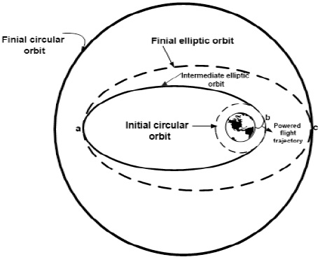
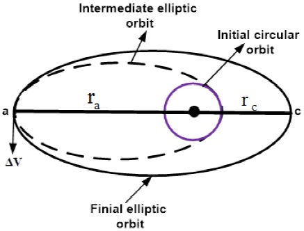
The flight sequence being considered is illustrated in Figure 1, and it is described as follows:
Power flight from the Earth’s surface to inject the spacecraft into a circular orbit at b, with radius rb.
At b, an impulsive velocity increment places the vehicle in an elliptic orbit of apogee ra and perigee radius rb.
At a, an impulsive velocity increment places the vehicle in a new elliptic orbit of apogee rc and perigee ra.
2.2. Equations of the transfer maneuver
1. On the initial circular orbit, the velocity is:
where µ is the gravitational constant equal to 398598.62 km3 / sec2.
2.On the intermediate elliptic orbit the velocity is Vb at point b and Va at point a. Since 2a = ra + rb, we get
that is,
3. The required impulsive velocity to inject the spacecraft into the intermediate elliptical orbit is:
Using Equation (4) we get
4. The required impulsive velocity to inject the spacecraft into the final elliptical orbit is:
since
using this equation and Equation (5), we get
5. On the final elliptical orbit, at the point c, the velocity is:
6. The required impulsive velocity to circularize the orbit, at point c, is:
2.3. Velocity requirements for the final transfer maneuver
From the above formulations, the expressions for the velocity requirements for the two cases of elliptical and circular final orbits will be obtained.
2.3.1. Velocity requirements for the final elliptical orbit
which is written as:
2.3.2. Velocity requirements for the final circular orbit
which is written as:
where
The positive sign in Equation (16) is used if α < β, while the negative sign is used for α > β.
3. Optimum mode of transfer
Having obtained the velocity requirements for the final elliptical and circular orbits, then, by comparing the energy (velocity), of the various modes of transfers, the most efficient method of injecting a vehicle into the final orbit could be decided. In this respect, some findings are to be established and listed as separated results.
3.1. The case for which α = β
The point of the intersection of the two curves ΔVTc /VCb and ΔVTe /VCb occurs according to Equation (16) when
that is, for all α = β, i.e. ra = rc, so we have:
Result 1: The two curves ΔVTc /V Cb and ΔVTe /VCb of equal values of β intersect at values of α, which is coincident with the value of β. From the transfer mode point of view, we have the result:
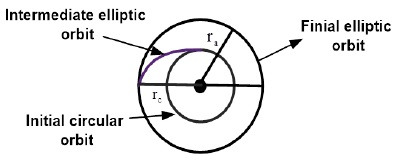
Result 2: Each of the points of intersection of the two curves ΔVTc /VCb and ΔVTe /VCb represents the case of a transfer from the parking orbit directly to the new orbit, and circularizing it at the end of the maneuver. This mode of transfer is illustrated in Figure 2.
For α = β, Equation (14) could be written as
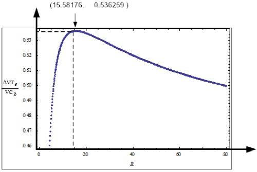
The graphical representation of Equation (19) is shown in Figure 3.
To find the maximum value of ΔVTe / VCb, it is necessary to differentiate Equation (19) with respect to α and equate the result to zero. We get
Multiplying both sides of this equation by √2(1 + α)3/2 α3/2 and then squaring it, we obtain
In Equation (21) there is only one change in the sign of the coefficients. Then, according to Descartes’ rule, there exists only one real root. This root is:
The maximum value of ΔVTe / VCb is, therefore
This ratio shows that the maximum ΔVTe is more than half of VCb, which is too expensive.
Result 3: For α = β, the velocity requirement of a circular orbit is of the maximum value 0.536258 at α = αM = 15.58176.
Now, let us consider the case where α → ∞. For this case we have, from Equation (19), that the velocity increment to escape to infinity is given by:
Also, the velocity to return from infinity, or equivalently the velocity to make the spacecraft to escape to infinity from its orbit, is given by:
The non-dimensional velocity increment for the total maneuver can be obtained by adding Equations (24) and (25), to get:
To determinate the point of intersection of the two curves ΔVTe / VCb and ΔV ∞/VCb, it possible to equate Equations (19) and (26), to get
Multiplying by √α and squaring both sides of the resulting equation, we obtain
that is
Multiplying by α + 1 and squaring both sides of the resulting equation, we get,
Hence, the required equiation is:
In Equation (31) there are three changes in the sign of the coefficients. Then, according to Descartes’ rule, this implies that there exist three real roots. These roots are: α = 0.146554; α = 0.571535; α = 11.93876. The first two roots are rejected, since we consider the case in which α > 1, so the only root in our case is:
The values of αM and αI of Equations (22) and (32), respectively, are used to study the superiority of circular or elliptic transfer maneuvers. Figure 4 shows the superposition of the two curves ΔVTe / VCb and ΔV ∞/VCb.
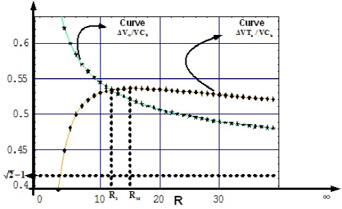
Result 4: The two curves ΔVTe / VCb and ΔV ∞/VCb intersect at (11.94, 0.534).
3.2. The case for which α ≠ β
To examine the case in which β > α, let β = α + ε, where ε is a real positive number that is less than one. Then, Equation (16) becomes
Thus, we get the following result:
Result 5: For all β > α, the velocity requirement for a circular orbit is always greater than for an elliptic orbit, but the difference approaches zero as β approaches infinity, which means an escape orbit.
For eccentric orbits, the least amount of energy is expended by transferring directly from the parking orbit to the apogee of the orbit, and then applying the necessary impulse to obtain the desired perigee. In all cases the energy requirements is lowest when β < α. For example, for α = 10 and β = 2,
But, for α = 2 and β = 10, we have
Table 1 illustrates Result 5 and its consequences. The type of transfer is represented in Figure 5.
Table 1 Result 5 and its consequences
| α | β | ΔVTe / VCb | α | β | ΔVTe / /VCb |
|---|---|---|---|---|---|
| 5 | 4 | 0.454433 | 4 | 5 | 0.475730 |
| 7 | 3 | 0.426663 | 3 | 7 | 0.499627 |
| 9 | 5 | 0.474288 | 5 | 9 | 0.539888 |
| 13 | 6 | 0.478357 | 6 | 13 | 0.568656 |
For circular orbits, in all cases the minima for β < αM occur either for α = 1 or α = β, which means that, for this range of β, it is more efficient to transfer directly to the final orbit and circularize it.
-
In the cases of minima for β > αM, it is more efficient:
To inject the vehicle into an elliptic orbit whose apogee is greater than the final circular orbit altitude.
Having reached the apogee, add an incremental velocity, which would raise the perigee to the final circular orbit altitude.
Upon reaching perigee, decelerate the vehicle to circularize its orbit.
3.2.1. The extreme values of ΔVTc / VCb
Equation (16) could be written as:
where R* = α and R = β. Also, we consider the case
Equation (36) contains two parameters, R and R*. For a fixed R, it gives an equation in R*, which should be possessed of maxima and minima. To obtain the extreme parametric members of this family of curves, let Equation (36) be differentiated with respect to R* and equate the result to zero. This could be performed as follows.
Differentiating Equation (36) with respect to R* we get:
Equating to zero we get
Where
And
Then
Where
Squaring both sides of Equation (42), we get the solution:
Furthermore, since the numerator is negative, the negative sign in the denominator is necessary in order that R∗ > 0. Therefore, for our case, we should have:
Since for the case under investigation R∗ > R > 1, it follows, from Equation (46) and the inequality (37), that:
That is:
Squaring the result, we obtain
Rejecting the physically impossible root R = −1/3, we have
which is the same as Equation (21). Therefore, this leads us to the result shown below.
Result 6: The limiting value of R for elliptic transfer is RM = 15.58176.
Equation (46) becomes unbounded for the condition:
which has real root R = 9. Consequently we have the result shown below.
From the above, it is clear that, the elliptic transfer can not be used for all R in the range (1, 9), thus we get the following result:
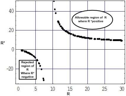
Result 7: The forbidden range for the elliptic transfer is
Result 7 is shown in Figure 6, with respect to R*.
3.2.2. Comparison between elliptic and circular transfers
From the above analysis, there exist two critical ratios, namely, RM and RI. In terms of these ratios and
Result 9, we have four inequalities:
where R I = αI = 11.938655. In what follows we shall discuss superiority of circular or elliptic transfers in each range.
The range: 1 < R < 9
According to Result 7, we have the result shown below.
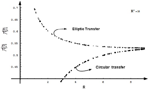
Result 8: For all R belonging to the range 1 < R < 9, and for all R* > R, circular transfer is superior to the elliptic transfer. This range is suitable, for example, in trajectories of flights to Venus and Mars. Typical graphical illustration of Result 8 is shown in Figure 7.
The range: 9 ≤ R ≤ RI
As in the above case, we have the result shown next.
Result 9: For all R belonging to the range 9 ≤ R ≤ RI, and for all R* > R, circular transfer is superior to the elliptic transfer.
Typical graphical illustration of Result 9 is shown in Figure 8.
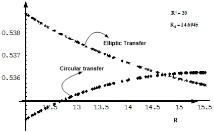
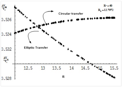
The range: RI ≤ R ≤ RM
In the range RI ≤ R ≤ RM, the two curves ΔVTe and ΔVTc / VCb intersect at R = R0 (say) for all values of R* > R. for a given value of R* > R, we can solve the equation.
numerically to find R0.
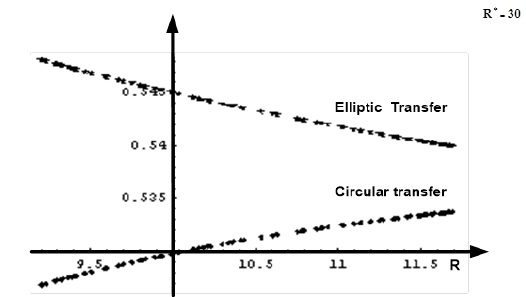
Result 10: For all R belonging to the range RI ≤ R ≤ RM and for all R∗ > R, then:
Circular transfer is superior to the elliptic transfer for all R < R0,
Elliptic transfer is superior to the circular transfer for all R > R0, where R0 is the root of Equation (54). Typical graphical illustrations of Result 10 are shown in Figures 9 and 10.
At this point, it should be noted that the most critical factor of a transfer maneuver is its duration time, especially for supplying space stations and space rescue operations. It is known that the motion in parabolic orbits possesses definite advantages, namely, it gives a gain in time, i.e. the duration of the flight will be significantly smaller. As, for example, the duration of flight from the Earth to Pluto, in the case of the parabolic trajectory, is 19.33 years, while the corresponding time in the case of the Hohmann trajectory is 45.60 years (Gurzadyan, 1996). However, a parabolic orbit requires an initial velocity √2 times greater than that for the corresponding elliptic orbit and, therefore, from the energetic point of view, parabolic orbits are not preferable, since we need a rocket that is more powerful and spends more energy.
The optimality of parabolic orbits with respect to the duration of flight, as mentioned above, tempted some authors to propose successful maneuvers containing parabolic transfer. One of these proposals is the elliptic-biparabolic planar transfer for artificial satellites developed by Prado (2003). The objective of this maneuver is to find the minimum cost trajectory, in terms of fuel consumed, to transfer a spacecraft from a parking orbit around a planet to an orbit around a natural satellite of this planet, or to a higher orbit around the planet. Moreover, the idea of using a natural satellite in the maneuver is applied to the problem of causing a spacecraft to escape from the main planet to interplanetary space with maximum velocity at infinity.
4. Conclusions
The problem of impulsive maneuvers for space missions is addressed, by considering the case of planar maneuvers with newly derived equations. In this regard, an analysis of the transfer maneuvers from initial circular orbit to a final circular or elliptic orbit is developed. Comparisons of circular and elliptic maneuvers, which are important for mission designers, are made. Useful mappings showing where one maneuver is better than another are shown. In this respect, we developed these comparisons throughout ten results, together with some graphs to show their meaning.

