1. Introduction

The cool, molecule-rich outer envelopes of a young planetary nebula (PN) seem to be an archive of its mass-loss history, which can date back from several thousands to several tens of thousands of years into the “superwind” phase of the former extreme AGB star, since ideally the density structure of the outer envelopes remains undisturbed by the hot wind and U V radiation that occur during the formation process of the PN. Obviously, a study of that archive should focus on the envelope out-side the optical (H_α) image of the PN. In an earlier work (^{Verbena et al. 2011}), we used the results from self-consistent models of similar dust-driven winds to show,using the continuity equation, that such an undisturbed density profile should be dominated by mass-loss changes and its subsequent dilution while changes in the wind velocity have only a minor impact.

Before the planetary nebula (PN) phase, and while a star is on the upper end of the asymptotic giant branch (AGB), it goes through a process of strong mass-loss, caused by the formation of dust and its subsequent acceleration due to the radiation pressure from the star. The evolution of the mass-loss process is shaped, over long time-scales, by the evolution of the stellar parameters (increase of the mass-loss rates as gravity and effective temperature decrease), and, over short time scales, by the fluctuations of the late AGB star following its thermal pulses or shell He-flashes.

After the star leaves the AGB, the dense, slow, dust-driven wind ceases, and is replaced by a fast, thin and very hot wind, accompanied by a hot U V radiation field, both stemming from the now exposed hot core of the former giant star. Wind and radiation begin to interact with the cool wind envelope ejected before, and create the optical appearance of the PN. Inside it, the shell material emits emission lines that cool and balance the radiative energy input; an inner shock-front (the inner rim of the optical PN) marks the extent of the mechanical impact of the hot wind, while the ionization-limit of the central star’s radiation field marks the outer rim. Unfortunately, the transition from the AGB to the young PN is short-lived (≈ 10³ yrs) and such objects are therefore difficult to find and observe directly.

After the hot central star has begun to ionize its surroundings, the ionization front moves ahead of the wind-collision region, disturbing the old density and local pressure profiles. With time, it may reach deep inside the outermost material, causing a D-type ionization front to advance into the inner portions of the AGB envelope, wiping out much of the evidence of later phases of AGB mass-loss. Hence, for the purpose of this study it was important to select a young, still compact PN. We also wanted to minimize as much as possible any complications introduced by a strong bipolarity.

In order to perform a quantitative density analysis, which included determining the excitation, of an AGB halo outside the extent of the optical PN, we made observations of the mostly optically thin ¹³CO in its two fundamental rotational transitions, J=1-0 and J=2-1 at 2.7 and 1.3 mm, respectively. Most of the mass in an AGB envelope consists of molecular hydrogen (H₂). However, a direct observation of that molecule is very difficult. because vibrational transitions get excited at much higher temperatures than those found in the cool outer envelopes of PNe. ^{Bremer et al. (2003)} did observe H₂ lines using ORFEUS-SPAS II spectra; these lines indicate the presence of H₂ and that it is likely associated with the nebula rather than with the intervening galactic gas. The present study focuses on the second-most abundant molecule, CO, in its optically thin isotopic variant (¹³CO). Since low quantum number transitions of this molecule become excited at relatively low temperatures (of the order of 10 K),we performed a representative probe of its density profile.

We used the results from concrete evolution models with strong mass-loss. The mass-loss histories derived from these models were diluted by the continuity equation, assuming for simplicity a constant expansion velocity for the entire halo. This allowed us to avoid complex hydrodynamical considerations in this first approximation to the problem. Indeed, the outflow velocity of a dust-driven wind does not vary too much on short time-scales (i.e., during and after thermal pulses). We published a more detailed report in ^{Verbena et al. (2011)}. Using the same simple approach (assuming a constant expansion velocity) we found a good agreement between observational and theoretical density profiles in a qualitative comparision; that is, the observed density slopes matched our models. However, without an absolute measure of the halo density, we could not confirm the mass-loss rates as such, only their relative changes over time during the final (“superwind”) phase (^{Phillips et al. 2009}).

¹²CO has already been observed in PNe (^{Dayal & Bieging 1996}), as it generates much stronger emission line profiles. In this work, however, the emphasis was on obtaining accurate, quantitative evidence of the density profile, where the much fainter but optically thin variant of the CO molecule is of great advantage. However, it is necessary to consider a few complications besides the need for a much larger integration time.

It has been pointed out that although an LTE analysis may (or may not) be valid for CO, the same cannot be said about its isotopic variants such as ¹³CO (^{Leung & Liszt 1976}; ^{Padoan et al. 2000}) due to uncertainties in the excitation temperature. Furthermore, even though CO might be easily thermalized, the same is not true for its isotopic variants; if an excitation temperature represents the level populations of the lower levels, it will not necessarily represent higher levels, given the higher Einstein coefficient, which means a faster depopulation. For this reason we performed a non-LTE analysis of the chemical state and temperature structure using the CLOUDY photonionization code. (^{Ferland et al. 2013}). We then used the RATRAN code to model the coupled problem of level population and radiative transfer in the halo (^{Hogerheijde & van der Tak 2000}). CLOUDY uses the escape probability approximation to the line transfer problem and could potentially be applied to the whole problem. But such a treatment assumes that the local mean radiation field is determined by local conditions alone, whereas RATRAN uses a Lambda-accelerated Monte Carlo method to solve the statistical equilibrium and the local mean radiation field as a coupled and non-local problem. We therefore consider this approach to be much more complete and used RATRAN to calculate the line transfer.

In the following, we first describe the observations and their results. In § 3.2, we compare the observational evidence (observed line emissions) with homogeneous halo models (constant density and constant kinetic temperature), then with (§ 3.3) density profiles prescribed by a power law of the form nr=10nirri-β, where n(r) is the density at the radius r, and n_i is the density at the density at the inner radius r_i; finally, we compare it (§ 3.4) with density profiles derived from mass-loss histories of concrete evolution models.

2. Iram observations of ¹³CO emission from the halo of NGC 6826

We made observations of the outer halo of NGC 6826 using the IRAM 30m telescope located at Sierra Nevada, Spain¹ in June 2011. The basic information of NGC 6826 is given in Table 1. Since there were no previous observation of ¹³CO towards this source, the integration time was estimated based on the CO observations of a proto-PN OH 231.8+4.2, which has a similar size and distance as our object of interest (^{Sánchez-Contreras et al. 1997}). From the outer-most position in map, we estimated an integration time of about 10 hours per pointing by extrapolating the strengths of the ¹²CO and ¹³CO lines and assuming that the ratio of the respective line strengths does not vary much with radial distance from the central star. In order to obtain basic density profile information from a small number of pointings of a necessarily very long integration time, we chose two representative positions in the outer halo of the planetary nebula NGC 6826 that were 60^′′ and 75^′′ away from the central star in declination. Table 2 shows the pointing positions and their respective integration times in hours. The positions can also be seen in Figure 1.

Table 1 Coordinates and basic information of the PN NGC 6826ngc 6826. 

NGC 6826
Right ascension	19h 44m 48.1501s
Declination	+50◦ 31’ 30.264”
vLSR	8.6 km/s
Distancea	1.1 kpc
Expansion velocityb	11 km/s

^{a Surendiranath & Pottash (2008)}.

^{b Guerrero et al. (1998)}.

Table 2 Observing time in hours for both positions. 

Band (GHz)	Integration time (hours)a
	60′′	75′′
110	6	10
220	8,4.3	12,7

^a The second number after the comma is the approximate final source time (ON+OFF) after editing the data.

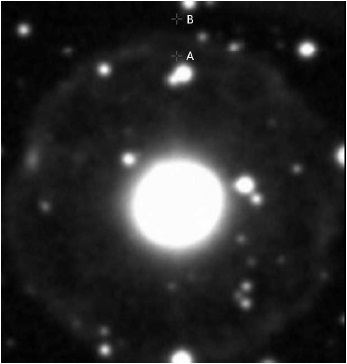
Fig. 1 Image of NGC 6826. Pointing positions labeled A and B at 60^′′ and 75^′′ from the central star. 

The observations were made at an elevation of about 50° and at a velocity, with respect to the local standard of rest, of v_lsr = 8.6 km/s. The frontend used was EMIR² (Eight MIxer Receiver), which allows simultaneous observations of the ¹³CO(1-0) and ¹³CO(2-1) lines. The backend used was VESPA³ (VErsatile SPectrometer Array). Each line was observed with a bandwidth of 120 MHz and a resolution of 80 kHz (≈ 0.2 km/s for J=1-0 and ≈ 0.1 km/s for J=2-1). We used the wobbler switching observing mode with the maximum extent of 2 arcminutes. The pointing of the antenna was regularly verified with strong continuum sources close to our object; thus, we expect it to be sufficiently accurate.

All data reduction was performed using the CLASS package, which is itself a part of the GILDAS (Groenoble Image and Line Data AnalisyS) analysis package (^{Pety 2005}). Line calibration was verified with the source DR-21, a giant molecular cloud in Cygnus, using a catalogue of calibrated spectra (^{Mauersberger et al. 1989}). The very long integration time of each pointing was acquired by a number of read-outs of shorter integrations of 9.5 minutes. Individual readouts affected by instrumental glitches and bad weather (i.e., variable water vapor content) were discarded before averaging the data. Thus, the effective ON source time was smaller than that given in Table 2. The resulting spectra were then smoothed to a resolution of ≈ 1.7 km/s for J=1-0 and ≈ 0.8 km/s for J=2-1 transitions respectively. The spectra were converted from TA* to T_mb units using forward efficiencies of 0.95 and 0.86 and beam efficiencies of 0.75 and 0.55 for 110 and 220 GHz (2.7 and 1.3 mm), respectively, as found by CLASS.

The beamwidth of the antenna was 11^′′ for the 110 GHz ¹³CO(1-0) transition, and 22^′′ for the 220 GHz ¹³CO(2-1) transition which translated into a physical size, considering a distance of 1.1 kpc, of 0.06 and 0.11 pc respectively. The pointings of 60^′′ and 75^′′ translated then into a physical distance of 0.32 and 0.4 pc from the central star of the PN. It is worth noting that the distance to NGC 6826 is not well known. Statistical distances range between 0.7 and 1.6 kpc. The distance of 1.1 kpc that we used was that obtained by ^{Surendiranath & Potasch (2008)} by equating the rms density with the forbidden line density, and is well within the range of statistical ditances.

We detected the lines of both transitions for the innermost pointing. The ¹³CO(1-0) and ¹³CO(2-1) transitions were detected at 2 and 1.7 σ levels respectively. No line was detected for the outermost point. However, we were able to estimate an upper limit for the line strengths using the rms of the spectrum. Figures 2 and 3 show the final spectra obtained using IRAM. The observed line properties are given in Table 3. Although it is not unexpected to detect a weak, narrow ¹³CO emission at the galactic latitude of the nebula, we believe this emission comes from the outer halo of NGC 6826, since 15^′′ away from our inner pointing we had no detection even after using a longer integration time.

Fig. 2 Spectra obtained at 60^′′ from the central star. ¹³CO(1-0) and ¹³CO(2-1). 

Fig. 3 Spectra obtained at 75^′′ from the central star. ¹³CO(1-0) and ¹³CO(2-1). 

Table 3 Properties of the observed lines. 

Line	Expected rms	Observed rms	Observed intensitya (K)
13CO(1-0) A	3.03 × 10−3	5.677 × 10−3	1.16168 × 10−2
13CO(2-1) A	3.03 × 10−3	9.523 × 10−3	1.56691× 10−2
13CO(1-0) B	8.31 × 10−3	8.992 × 10−3	2.182 × 10−3
13CO(2-1) B	8.31 × 10−3	1.031 × 10−2	10−3

^aFor point B, we show the rms observed in the line window.

3. Halo density profile: modelling of the ¹³CO observations

The morphology of the the PN NGC 6826 seems spherical, as can be seen on the Hα+[NII] images of ^{Corradi et al. (2003)}. The source has an inner region filled with ionized gas and an outer spherical halo. The ¹³CO molecular emission is expected to come from the outer halo. The analysis of observations made by ^{Corradi et al. (2003)} showed that the inner radius of the dusty halo is about 4 × 10¹⁷ cm, and that the outer radius is about 1.8×10¹⁸ cm from the central star. Assuming these parameters for the halo, we modeled the ¹³CO line observations, in order to constrain the density and temperature profile of the halo. In the following, the line emissions observed from the outer envelope of the PN NGC 6826 are first interpreted as a simplified halo with homogeneous density and temperature, then as physically more realistic models of a photo-dissociation region (PDR) with a prescribed density profile in which the radial profiles of temperature and molecular abundance are constrained by the model.

3.2. Homogeneous halo: non - LTE model

Given the low densities estimated from the simplified LTE analysis of the ¹³CO observations above, we expected the line intensities to be affected by non-LTE effects. Therefore, we used non-LTE models to interpret the observations. In order to understand the role of non- LTE effects, we started by considering a halo of homogeneous density and temperature. The excitation temperature and line intensities were calculated using the radiative transfer code RATRAN (^{Hogerheijde & van der Tak 2000}), always with the LAMDA molecular database (^{Schöier 2005}). This analysis was performed for a range of temperatures (between 10 and 1500 K) and densities (from 10^0.5 to 10³ cm⁻³). The line intensities of the homogeneous models are plotted in Figure 4 as contours for different values of the logarithmic line intensities (in K).

Fig. 4 Contour plot of line intensities (as given by logarithmic antenna temperature in K) for homogeneous halo models, using RATRAN, and adopting a ¹³CO/H₂ molecular abundance ratio as given in § 3.1. The left and right panels show the contour plot for the J=1-0 and J=2-1 transitions, respectively. 

The observed line intensities towards pointing A suggest a density of about or above ≈ 3.5 cm⁻³, and a temperature between 10 and −30 K. However, the upper limits of the line intensities obtained towards pointing B suggest a much lower density and temperature. These results again indicate the existence of a density profile in the halo, rather than a homogeneous density.

3.3. Halo with a variable density profile: PDR models

In a more realistic model with variable density and temperature profiles, the far-ultraviolet (FUV) radiation from the central star establishes a PDR in the molecular halo (^{Tielens & Hollenbach 1985}). Thus, at any point in the halo, the temperature and the ¹³CO molecular abundance are not free parameters, but are physically constrained by the chemistry and respective radiative cooling and heating rates in the PDR.

We modelled the halo as a PDR using the CLOUDY code. The input of the PDR models consisted of the radiation field from the central star at the inner radius of the spherical halo, and the density profile in the halo. The stellar parameters of the central star were taken from ^{Balick et al. (1998)}. We also included a simple interstellar radiation field, as described in ^{Draine & Bertoldi (1996)}, as well as the CMB.

The halo density distribution is prescribed by a simple power law of the form:

nr=10nir-β (1)

where n(r) is the density at the radius r, n_i is the density at the inner radius r_i, and the exponent β models the radial decline. For these calculations, the elemental abundances were taken from ^{Surendiranath & Pottasch (2008)}. Furthermore, these CLOUDY calculations consider the warm dust continuum of the dust grains of a typical ISM and the PAHs (^{Mathis et al. 1977}). Our CLOUDY runs yielded temperature and abundance profiles for each model. The H₂ and ¹³CO abundances were of special interest for us; we used them as input to the RATRAN code to solve the line radiative transfer problem using the LAMDA molecular database (^{Schöier 2005}).

We built over 200 models to compare their results with the observed line intensities. The range of calculated models covered a parameter space of n_i from 1 to 5.5 and β from 0 (constant density) to 4 (steepest slope). Figure 5 shows contour plots based on these results; they are similiar to those of Figure 4, except that now the line intensities are a function of the initial density n_i and the β parameter.

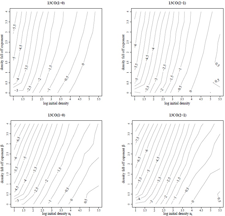
Fig. 5 Contour map showing line intensities (given by logarithmic antenna temperature in K) as predicted by halo densities following a simple power-law, nr=10nir-β, over a range of n_i, and β values for the pointings taken at a radial distance of 60^′′ (top) and 75^′′ (bottom). 

In order to constrain the best fitting n_i and β values, we plotted the observed line intensities and the χ² contours in Figure 6. The colors white, light grey and dark grey, indicate confidence levels of 63%, 95% and 99%, respectively. We could constrain the parameter n_i (between about 2 and 3.5), but because of the non-detection at the outer point, it was more difficult to constrain β.

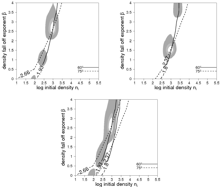
Fig. 6 χ² contour plots for the line emissions in the two pointings. The top left plot is for the ¹³CO(1-0), the top right one for the ¹³CO(2-1) line, and the bottom one is for both lines together. The white areas within the contour represent a confidence level of above 63%, the light grey of 95%, and the dark grey of 99%. Solid lines represent the respective χ² contours at 60^′′, dotted lines at 75^′′. 

Consequently, we used a different method to con-strain the β parameter. The emerging line intensities can be calculated for any point in the envelope for any given density and temperature profile. This allowed us to plot the line intensities as a function of the distance from the center (see Figure 7) and to compare them directly with the observed intensity at 60^′′ and the upper limit at 75^′′. Using a β = 0.5 (first plot from the left in Figure 6) yielded an intensity slope that was too shallow. In other words, the outer pointing should have resulted in a detection. Acceptable slopes (consistent with a non-detection in the outer halo pointing) are found above a value of β of 2.5, as can be seen in the bottom panel in Figure 6. These plots provide a further constraint of β≳2.5.

Fig. 7 Line intensity (given by antenna temperature in K) as a function of the distance to the central star in arcseconds for different values of n_i. The dotted lines correspond to the J=1-0 transition and the solid lines to the J=2-1 transition. The dots represent the actual observations: • J=1-0, ◦ J=2-1. The arrows on the observations at 75^′′ indicate that this is an upper limit. 

In Figure 8 the radial dependence of the line intensities is plotted for different β values and different densities, corresponding to the 68% confidence region of the best fit. The top panels show the J=1-0 observations and also show that the best fit-ting model allows densities of n_i = 3, β > 3. Similarly, using the results of the J=2-1 transition shown in the bottom panels allowed density values higher than 3.

Fig. 8 Line intensities versus radial distance, observed (dots) and calculated for the ¹³CO(1-0) (top), and ¹³CO(2-1) (bottom) lines with density-laws with 2.5 < n_i < 3.5 and 2.5 < β < 3.5. 

3.4. Density profiles from mass-loss histories of evolution models

To test the validity of our evolution models with strong mass loss in the final AGB “superwind” phase, we performed an analysis using density pro-files derived directly from mass-loss histories obtained in those conditions. We used the results of our well-tested and calibrated evolution code based on the work of ^{Eggleton (1971}, ¹⁹⁷², ¹⁹⁷³), which was updated and described by ^{Pols et al. (1998)}, and combined with a parameterized mass-loss prescription for dust-driven winds as described by ^{Wachter et al. (2002)}. The most appropriate mass-loss history was derived from an evolution model of a star with an initial mass of 2.25M_⊙. As mentioned above, the resulting density profile was derived by applying the following the continuity equation:

ρ=dMdt14πr2v (2)

where dM/dt is the mass-loss rate at a given time, r is the radius and v is the expansion velocity, which we consider to be approximately constant (^{Verbena et al. 2011}). The radius was obtained by multiplying the expansion velocity by the dynamical age of the nebula shell. This approach has already been used by us to make a qualitative comparison between density profiles and observations (^{Phillips et al. 2009}), in which we looked only at the slopes of the emissions; a quantitative test is still needed to obtain appropriate observational evidence.

Figure 9 shows the density and temperature profiles given by CLOUDY, as well as the lines that fit them (broken lines). The comparison was done between mass-loss histories with initial masses of 1.25 and 2.25M_⊙ and varying the age over several thousands of years. A mass of 2.25M_⊙ and an age of 3900 years gave the best fit, i.e., the results had the lowest t-value in the χ² analysis.

Fig. 9 The two top graphs show the density and temperature profiles used for the best line-fitting model. The density profiles were derived from the mass-loss history of our evolution model for M_i = 2.25M_⊙, and the temperature profiles were subsequently computed by RATRAN. The bottom graphs show the resulting model line profiles (in red) over the observed ¹³CO(1-0) (left) and ¹³CO(2-1) (right) lines. The color figure can be viewed online. 

4. Discussion and conclusions

Observations of ¹³CO(1-0) and ¹³CO(2-1) lines in the halo of the PN NGC 6828 at radial distances of 60^′′ and 75^′′ from the central star resulted in a good detection at the inner pointing, but only in the establishment of upper limits to the observed fluxes at the outer pointing. We interpreted the detection of ¹³CO and the upper limits using first a simplified, homogeneous halo in LTE. These results supported the existence of a density gradient, as well as the necessity of considering non-LTE effects. Consequently, we then applied the physically more realistic approach of using non-LTE RATRAN and CLOUDY models of a PDR with different, prescribed density profiles, where the temperature and molecular structure were defined for each point of the envelope by the balance between the radiation field and the respective radiative cooling.

The lack of detection in the outermost point also limited the results presented here. We used the rms as upper limits; thus, it is possible that the intensity at the outermost point is actually much lower. We only considered models with slopes that represent density profiles well below this point. It is unlikely that the slopes are much smaller, given that all stellar evolution models result in a mass-loss history that would not suggest such a low density. If indeed the density were much smaller, we would have a shell with a different age for the shell, or a much higher initial mass. Higher mass models result in more abrupt changes in mass-loss rates, which translate into steeper density profiles. In the worst case scenario, we would need to assume a totally different mass-loss rate and wind prescription deviating from what is expected from evolution models. We conclude that it is important to continue making observations of this and other suitable objects to either support or refute our conclusion and to refine our evolution and wind models.

In the semi-empirical approach, the PDR-models that best matched the observed line profiles and intensities, as well as the upper limits of the outer pointing, suggest that the halo has a decreasing density profile with a power law exponent β > 3 and a density at the inner radius of about 300 < n < 3000 cm⁻³.

The observed line intensities can also be fitted by theory-based PDR models that use the same density and temperature profiles predicted by our mass-loss history models for a different stellar initial mass, under the simple assumption of an approximately continuous outflow. A density profile of the outer envelope of the PN produced by the mass-loss history of a concrete evolution model (2.25M_⊙) gave the best match to our observational results.

We chose NGC 6826 as an ideal candidate, due to its shape and giant halo. We assumed that there was molecular material in the outer halo that we could use to probe into the nebula’s previous mass-loss history. The use of CLOUDY allowed us to take into account the interstellar radiation field and the stellar U V emission in order to obtain the molecular abundances that we needed to trace the ¹³CO emission lines. ^{Middlemass et al. (1989)} observed the nebula through visible emission lines and obtained the electron density and electron temperature of the halo; the latter was even higher than that of the core. Our results seem to be in contradiction with theirs, but the ¹³CO emission lines indicate that there is indeed molecular gas within the halo. We would like to make a more extensive analysis of this and several other PNe to investigate further this apparent contradiction.

We are also aware that a more realistic approach should consider a varying expansion velocity, as well as the interaction of the halo material with the ISM. However, that would require complex and CPU-time consuming hydrodynamical computations, which may not provide a unique answer given the complex parameter space. For this reason, we consider the rather simple approach described here and its semi-empirical results as a good approximation to this complex problem. It could serve as a guide to build other, more refined, models.

Recent observations in the infrared by the Planck collaboration (Arnaud et al. 2015), have been associated with AGB mass-loss histories, and one of the objects of study was NGC 6826; however, they also considered a constant mass-loss rate during the AGB, which was reflected in the dependence of the density distribution on r⁻², whereas the mass-loss history we used was based on stellar evolution models and hydrodynamical models of stellar winds.