nueva página del texto (beta)
 Inglés (pdf)
 Artículo en XML
 Referencias del artículo
 Enviar artículo por email
 Citado por SciELO
  Similares en
SciELO
Similares en
SciELO 
 Permalink
1. INTRODUCTION
Integral Field Spectroscopy (IFS) is steadily becoming a common technique after several years of being limited to a handful of specialists across the world. In particular, IFS is nowadays widely used to study the spectroscopic properties of galaxies and their evolution along cosmological times. This is evident in the observational pattern that has evolved from studies focused on limited samples or individual objects (e.g. García-Lorenzo et al. 2005; Rosales-Ortega et al. 2011) to studies of large samples of galaxies in the last decade (e.g. González Delgado et al. 2015).
After the success of prototyping surveys, like SAURON (Bacon et al. 2001), a new set of observational programs has flourished, either at low redshift: e.g. Atlas3D (Cappellari et al. 2011), Disk Mass Survey (Bershady et al. 2010), CALIFA (Sánchez et al. 2012), and the on-going MaNGA (Bundy et al. 2015) and SAMI (Croom et al. 2012) surveys, or at high redshifts: e.g. SINS (Forster Schreiber et al. 2006). Despite their differences, like the number of galaxies observed and/or the number of spaxels sampling each galaxy, the total number of spectra of these surveys is similar, to order of magnitude, to the total number of spectra in the Sloan Digital Sky Survey (York et al. 2000), as recently highlighted by Sánchez (2015). Moreoever, the advent of new in strumentation able to produce even larger datasets for a single galaxy (e.g., MUSE Bacon et al. 2010), and their likely use in survey mode, will increase by orders of magnitude and very fast the number of IFS spectra to be analyzed. For this reason, it is necessary to develop new tools capable of analyzing spectra of different surveys in a consistent and automatic way.
In order to address this problem we developed P 3D. This article is the second in a series focused on the description of this pipeline, a spectroscopic analysis tool developed to characterize the properties of the stellar populations and ionized gas emission lines in the spatially resolved data of optical IFU surveys. In the first article of this series, (Sánchez et al. 2015 b, hereafter Paper I), we described in detail the basic fitting algorithms behind P 3D, included in a package named FIT3D. In that article we focused on the description of how the algorithms work on an individual spectrum, on the definition of the different parameters recovered, and on the estimation of the accuracy of the numerical values recovered, as well as on the limitations of the methodology. In the present article we focus on the description of how P 3D handles a complete datacube. We describe step-by-step the different analyses performed on the data to generate the dataproducts. In order to illustrate the process we use real data extracted from on-going IFS surveys.
The sequence of the article is as follows: In § 2 we describe the datasets that have been used to illustrate how the pipeline works. In § 3 we describe the full analysis process, step by step, including (i) the description of the pre-processing of the data, required to perform an homogeneous analysis for different datasets (§ 3.1); (ii) the analysis of the central spectrum (§ 3.2), with a detailed description of the study of the stellar population(! 3.2.1); (iii) the spatial binning scheme adopted in P 3D in order to increase the S/N of the stellar continuum, indicating the main differences with the most common used one (§ 3.3); (iv) the analysis of the stellar population in the different spatial-bins and the corresponding analysis of the emission lines (§ 3.4 and § 3.4.3); (v) the dezonification procedure and how a emission line pure datacube is generated (§ 3.4.4); (vi) the analysis of the stellar indices forthe spatially binned spectra (§ 3.6.1); (vii) § 3.5 and § 3.6 describe the procedures adopted to analyze the strong and weak emission lines spaxel-wise for the emission line datacube; (viii) § 3.7 summarizes the way the dataproducts are packed in a set of datacubes in order to be distributed in a simple way. (ix) A practical use of P 3D is described in § 4, including the distribution of all the dataproducts derived for the V500 setup of the CALIFA DR2 galaxies (Garcia-Benito et al. 2015); Finally, the summary and conclusions from this article are included in § 5.
2. DATA
Along this article we describe the different steps of the analysis pipeline illustrating the intermediate results using the following IFU data of the galaxy NGC 2916: (i) the datacubes provided by the CALIFA survey (Sánchez et al. 2012), in both the high and low spectral resolution modes, and (ii) the datacubes provided by the P-MaNGA studies (Bundy et al. 2015). This galaxy was selected since it was already used by Cid Fernandes et al. (2013) and Cid Fernandes et al. (2014) to illustrate the use of their own analysis pipeline, based on
The details of the CALIFA survey, the sample, observational strategy, and reduction are explained in Sánchez et al. (2012). All galaxies were observed using PMAS (Roth et al. 2005) in the PPAK configuration (Kelz et al. 2006), covering an hexagonal field of view (FoV) of 74"x64", which was sufficient to map the full optical extent of the galaxies up to two to three disk effective radii. This was possible because of the diameter selection of the sample (Walcher et al. 2014). The observing strategy guaranteed complete coverage of the FoV, with a final spatial resolution of FWHM≈2.5 ", corresponding to ≈1 kpc at the average redshift of the survey (García-Benito et al. 2015). The sampled wavelength range and spectroscopic resolution (3745-7500 Å. λ/∆λ ≈850, V500 setup) were more than sufficient to explore the most prominent ionized gas emission lines from [O ]λ3727 to [S ]λ6731 at the redshift of our targets, on one hand, and to deblend and subtract the underlying stellar population, on the other (e.g., Kehrig et al. 2012; Cid Fernandes et al. 2013, 2014; Sánchez et al. 2013, 2014). In addition the objects were observed us ing a higher resolution setup, covering only the blue end of the spectral range (3700-4800Å, λ/∆λ≈ 1650, V1200 setup). The exposure time in this second setup was three times larger than in the previous one to ensure a similar depth of the corresponding data. The dataset was reduced using version 1.5 of the CALIFA pipeline, whose modifications with respect to the ones presented in Sánchez et al. (2012) and Husemann et al. (2013) are described in detail in García-Benito et al. (2015). In summary, the data fulfilled the predicted quality-control requirements with a spectrophotometric accuracy better than a 6% in the entire wavelength range.
The details of the MaNGA survey, its sample, observational strategy, and reduction are explained in Bundy et al. (2015) and Law et al. (2015). The MaNGA instrument was developed under the framework of the SDSS-IV project. It deploys 17 science integral field units (IFUs), each one composed of an hexagonal array of fibers, across a field of view of 3 degree diameter attached to the 2.5m Sloan Telescope (Gunn et al. 2006). Individual science IFUs range in size from 19 fibers (12.5" diameter) to 127 fibers (32.5" diameter), with a diameter of 2"/fiber, and a 56% effective filling factor. The fiber-ends are coupled with the BOSS spectrographs (Smee et al. 2013), which provides a continuous wavelength coverage from 3600 Å to 10300 Å at a spectral resolution R≈2000 (R≈1600 at 4000Å, and R≈2300 at 8500Å), with a total system throughput of ≈25%. More details on the MaNGA setup are given by Drory et al. (2015).
The P-MaNGA, or MaNGA prototype, observations were obtained for three galaxy fields in January 2013, as a testing phase of the instrument, spectrograph, observing procedures, and data reduction. They comprise a heterogeneous sample of galaxies, including four objects selected from the CALIFA survey for photometric and astrometric calibration purposes: IC 0944, NGC 2916, UGC 05124, UGC 06036 (e.g. Bundy et al. 2015; Belfiore et al. 2015; Li et al. 2015; Wilkinson et al. 2015). Like in the case of the CALIFA survey, a three dithering scheme was adopted to obtain a complete spatial coverage, filling the gaps between the adjacent fibers. The raw data were reduced using a prototype of the MaNGA Data Reduction Pipeline (DRP), which is described in detail by Law et al. (in preparation). In essence, the data reduction includes all the usual steps required to extract the fiber-based spectra from the CCDs, perform the wavelength calibration, correct for the fiber-to-fiber transmission, subtract the sky spectrum, perform the flux calibration and re-arrange spatially the spectra (e.g. Sánchez 2006 a). The MaNGA and P-MaNGA data have the same spectral resolution, similar to CALIFA-V1200, and a spatial resolution similar to the CALIFA data (≈2.5", Bundy et al. 2015).
The final product of the data reduction from both surveys is a regular grid datacube, with x and y coordinates that indicate the right ascension and declination of the target, and the z coordinate a common step in wavelength, (in the case of CALIFA), or in the logarithm of the wavelength (in the case of P-MaNGA). For simplicity the P-MaNGA cubes were transformed to the same format of the CALIFA ones. In both cases the pipelines also provide the propagated error cube and a proper mask cube of bad pixels. In the case of CALIFA they also include a prescription to handle the errors when performing spatial binning (due to covariance between adjacent pixels after image reconstruction). Although we describe here the analysis of this particular dataset, which comprises galaxies in common between these two surveys, P 3D is capable of analyzing data from any of the three major on-going IFU surveys: MaNGA, CALIFA, and SAMI (Croom et al. 2012). There are very few galaxies in common between the three surveys, because although the red-shift footprints overlap, the sample selection criteria are quite different. In a companion article (Sánchez et al., in preparation) we will provide the dataproducts for the early-data release of the SAMI survey (Allen et al. 2015).
3. ANALYSIS SEQUENCE
P 3D analyzes each individual datacube in a fully automatic way, without using any additional external information on the object to be analyzed (like redshift, as-trometry, and so on). Here we describe the different individual steps taken and the dataproducts provided.
3.1. Cube pre-processing
Prior to any analysis, a preprocessing of the datacubes is required in order to (i) standardize the input format and (ii) determine which areas within the FoV of the data are suitable for the analysis.
Most IFU surveys, and in particular CALIFA, MaNGA, and SAMI, provide a FITS format file including a datacube as the final product of the reduction. In that cube, created using different interpolation/image-reconstruction schemes, the X and Y coordinates correspond to the spatial dimension (i.e., RA and DEC), and the third coordinate corresponds to the wavelength. All of them include several extensions in the FITS files that store, not only the physical flux intensity at each location and wavelength, but also the propagated error associated with those fluxes, a mask to indicate which pixels within the cube should or should not be taken into account, and finally even the weight of the covariance in the error propagation. However, the actual format is different for each survey (e.g., see Husemann et al. 2013; García-Benito et al. 2015, for a few examples). P 3D requires all the input cubes to be in the same format, which corresponds to the configuration adopted for the CALIFA datacubes, since it was originally developed for this survey.
The input file FITS format is described in Husemann et al. (2013), and it comprises a set of data cubes stored as extensions of the same file. The first extension corresponds to the measured flux densities, corrected for Galactic extinction in units of 10-16 erg s-1 cm-2 Å-1, with the wavelength solution following a linear step of a fixed spectral sampling (d λ). The second extension cor responds to the 1σ noise level of each pixel as formally propagated by the pipeline. Those two extensions are mandatory for P 3D. In addition, if there is a third extension it is identified as the bad-pixel mask, where the pixels not usable are indicated with a 1. Any further extensions will be ignored by the code.
Therefore, in the case of CALIFA data it is not necessary to perform any modification of the original cubes. But in MaNGA and SAMI there are different modifications that have to be taken into account. In the case of MaNGA the spectral sampling should be transformed from the logarithmic scale to a linear one (at least in the current format of the MaNGA data). Note that this transformation does not alter the spectral resolution of the data, nor does it fix it to a particular value. We have just re-sampled the data. In addition the order and meaning of the extensions should be re-arranged to produce the required input file. Finally, in the case of SAMI the blue and red datacubes correspond to two different and discontinuous spectral ranges (Croom et al. 2012), and should be glued into a single dataset to cover the maximum wavelength range observed by the final setup of this survey (3720-7426 Å). One should take into account that this final wavelength range is different from the largest accessible one by the SAMI instrument, due to the selected setup for the red spectra (Croom et al. 2012). The spectra included in the red datacube provided by the SAMI pipeline are degraded to the instrumental resolution of the blue datacube before creating a COMBO datacube. That procedure is mandatory if we want to analyze the blue and red-arm spectra together as a single spectrum per spaxel. Then the cubes are just combined by using the two datasets and interpolating the spectra to a common linear spectral sampling (adopting the one of the blue datacube). Obviously, the COMBO datacubes have a blank wavelength range between ≈5800 and ≈6300 Å. Finally, all the cubes are converted to the same flux units, 10-16 erg s_1 cm-2 Å-1 spaxel-1, to facilitate comparison of the results. The cubes are corrected for galactic extinction (when feasible) using the information in the header, the Milky Way extinction law by Cardelli et al. (1989), and a Milky Way specific dust attenuation of Rv =3.1.
The next step selects the areas of interest within the FoV. Due to the nature of the IFU systems provided by the three surveys, the useful FoV follows either a fixed hexagonal shape (CALIFA), an hexagonal shape of different size (MaNGA), or a circular shape (SAMI). Furthermore, in many cases the FoV covers foreground stars that should be masked, either using a proper catalog of field stars or a mask provided by the user. Finally due to the gradients in the surface brightness of galaxies across the FoV there are areas with too little S/N to perform any reliable analysis of the stellar continuum, even in the case of a proper spatial binning. Those areas should be masked for the analysis of the continuum, but not (in general) for the analysis of the emission lines, since the spatial pattern of both components (and therefore of the S/N distribution) are in general decoupled. In P 3D we mask all the areas with a S/N<3 in the wavelength range 5590-5680 Å. This range was selected to avoid possible contamination by night sky emission lines, and at the same time avoid moderate contamination by emission lines in the galaxy. This masking is needed since at low S/N the noise is not dominated by the Poissonian errors of the intensity of the astronomical target, but by other effects such as the sky brightness and sky subtraction, or by the electron noise, which require to perform a binning of a huge area to increase the S/N to an acceptable level. This is a problem, since at large areas the co-added spectra lack coherence in their properties, e.g., different kinematics, different stellar populations, and different sources of gas ionization may be present.
3.2. Analysis of the central spectrum
Initially the pipeline extracts the central spectrum of each datacube, defined as the 5" diameter (2.5" radius) aperture spectrum in the case of CALIFA (P-MaNGA), centred at the peak intensity in a broad-band image of the corresponding object. The broad-band image in the observed frame is synthesized by convolving the filter response curve through the datacube. For the CALIFA V500 and the P-MaNGA we use the V band filter, while for the CALIFA V1200 we use the B band. Figure 1 shows a comparison between the three broad-band images, illustrating the similarities in terms of spatial resolution between the three different datasets. The absolute flux intensities differ within the expectations for the CALIFA and P-MaNGA datasets. We must recall here that the current estimations of spectrophotometric accuracies for CALIFA are of the order of ≈ 3 - 4 % (García-Benito et al. 2015), while for P-MaNGA they are of the order of ≈ 15% (Belfiore et al. 2015). The lower photometric accuracy of the P-MaNGA observations arises because the prototype MaNGA hardware was designed to explore a variety of alternative flux calibration methods in order to determine the optimal approach for the main survey. In contrast, the full MaNGA survey-mode data reach spectrophotometric accuracies of ≈ 3% (Yan et al., submitted). The P-MaNGA datasets were originally reduced using a preliminary version of the pipeline, and therefore there are some inaccuracies associated with the reduction that are expected to be larger than those of the current version of the MaNGA datacubes (Law et al. 2015).
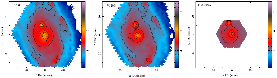
Fig. 1 Broad-band image maps synthesized from the V500 (V-band), V1200 (B-band) and P-MaNGA (V-band) datacubes in logarithmic scales of 10−16 erg s−1 cm−2 arcsec−1. The contours represent the intensity level starting at 10−17 erg s−1 cm−2 arcsec−1 and with successive steps of 10−17 erg s−1 cm−2 arcsec−1. The color figure can be viewed online.
An example of the central spectra extracted from each datacube is shown in Figure 2. For each spectrum we applied the stellar population and emission line fitting procedures described in Paper I (§ 2). First, each spectrum was fitted using a very simple template including two SSPs plus a spectrum of an emission line source, for the non-linear analysis, with the main aim of estimating the systemic velocity of the galaxy, its central velocity dispersion and the dust attenuation. In this first analysis a wide range of non-linear parameters is explored. A priori, the explored range of systemic velocities covers the full redshift range of the survey considered. The velocity dispersion covers the range between 0 and 400 km/s, including most of the known central velocity dispersion values for galaxies. Finally, the dust attenuation for the stellar population covers a range from Av=0 to 1.6 mag. This latter parameter is derived from the range of dust attenuation values observed in most galaxies (e.g. Charlot & Fall 2000; Calzetti 2001). The number of SSPs in this template is limited for the shake of speed, due to the strong dependence of the computational time on the number of SSPs in the template and on the range of parameters explored.
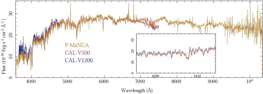
Fig. 2 Central spectrum of NGC2916 for 5" aperture centered on the peak emission of the galaxy extracted from the V500 (in red) and the V1200 (blue) CALIFA setups, and the P-MaNGA datacubes (orange). The inset shows a zoom area centered on the Hδ and Hγ spectral regions to highlight the similarities between the datasets. The color figure can be viewed online.
If there is a hint of the expected non-linear parameters, such as a published systemic velocity and velocity dispersion from previous analyses (e.g., from SDSS spectroscopy), or the expected dust attenuation, the pipeline can restrict the range of parameters explored and speed up the process.
After the non-linear parameters are derived, each spectrum is fitted, in the linear phase, with a limited stellar population library that includes 12 SSPs, as described below. This provides a simple but robust estimation of the properties of the stellar populations and the shape of the underlying continuum (e.g. Sánchez et al. 2013).
All SSP templates used so far, were extracted from the MILES project (Sánchez-Blázquez et al. 2006; Vazdekis et al. 2010; Falcón-Barroso et al. 2011). We selected this template on the basis of the results of Paper I, were we demonstrate that is is optimal for the analysis of the stellar population based on simulations (§3.1 and § 3.2 of that paper). The main reason is that it is based on one of the best spectrophotometrically calibrated libraries of stellar spectra. The template library adopted for the estimation of the non-linear parameters of the central spectrum of the galaxies comprises two extreme stellar populations: (i) a young (≈90 Myr) and low metallicity (Z/Z ʘ = 0.2) stellar population, and (ii) an old (≈ 17.8 Gyr) and high metallicity one (Z/Z ʘ = 1.5). In addition it includes an empirical spectrum characteristic of an emission line nebula, corresponding to the integrated spectrum across a Fo V of 5' x 6' of the Orion Nebula (Sánchez et al. 2007c). The choice of the spectra included in this template was the result of different experiments, guesses and errors along the past five years of analyzing CALIFA data, and nearly two years of analyzing MaNGA and SAMI data, in order to recover the non-linear parameters in a way consistent with the values reported for the central SDSS spectra (e.g. Mármol-Queraltó et al. 2011; Sánchez et al. 2012).
The template library adopted for the estimation of the properties of the stellar populations of the central spectrum comprises a grid of SSPs including four stellar ages (0.09, 0.45, 1.00, and 17.78 Gyr), and three metallicities (0.0004, 0.019, and 0.03), subsolar, solar, and supersolar. This template library, miles 12 hereafter, was used in many previous CALIFA studies, for instance, Sánchez et al. (2012, 2013, 2014) and Barrera-Ballesteros et al. (2015). Note that we use a very simple template library in this case since the main goal of the analysis of the central spectrum is to derive the systemic velocity and the central velocity dispersion properties. The results of the analysis of the stellar population is not used anymore by the pipeline, and the template is adopted just to speed-up the computing process.
3.2.1. Detailed analysis of the stellar population
After a first guess of the systemic velocity and the central velocity dispersion has been obtained (on the basis of the analysis described above), the procedure is repeated, restricting the exploration of the kinematic parameters within a range of ±300 km/s around the estimated systemic velocity, and ±50% around the estimated velocity dispersion. The dust attenuation is explored in the same range of values. For this second iteration we select a template with 3 SSPs for the non-linear exploration (i.e., the derivation of the velocity, velocity dispersion, and dust attenuation, as described in Paper I, § 2.1), including the two extreme populations described above and an intermediate population with an age of ≈1 Gyr and metallicity Z/Z ʘ = 0.4. For the linear exploration (i.e., the detailed analysis of the stellar population by a multi-SSP decomposition), a more complex stellar library was considered, defined as gsdl56 in Paper I (§ 3.1 of that paper). This library is described in detail in Cid Fernandes et al. (2013). It comprises 156 templates that cover 39 stellar ages (1 Myr to 13 Gyr), and 4 metallicities (Z/Z ʘ = 0.2,0.4,1, and 1.5). These templates were extracted from a combination of the synthetic stellar spectra from the GRANADA (Martins et al. 2005) and the SSP libraries provided by the MILES project. This SSP template has been extensively used by the CALIFA collaboration in different studies (e.g. Pérez et al. 2013; Cid Fernandes et al. 2013; González Delgado et al. 2014). The only difference with respect to these studies is that the spectral resolution of the library was not fixed to the spectral resolution of the CALIFA V500 setup data (FWHM≈6 Å), to allow its use for datasets with different resolution (like the ones provided by MaNGA and the CALIFA V1200 setup). This SSP-library uses the Salpeter (1955) initial mass function (IMF). Although the current implementation of the pipeline uses this SSP library, P 3D is not restricted to this particular one; it can be exchanged by modifying a configuration parameter in the main script.
As described in Paper I, § 2, FIT3D allows to fit the stellar continuum and the emission lines by means of an iterative procedure. In the case of P 3D we fit the strongest emission lines in the optical wavelength range, jointly fitting the following emission lines: (i) [O ]λ3727; (ii) Hδ; (iii) Hγ; (iv) Hβ, [O ]λ4959, and [O ]λ5007; (v) [N ]λ6548, Hα, [N ]λ6583, [S ]λ6717, and [S ]λ6731. In this way, we define a set of wavelength ranges including the indicated set of emission lines, and they are all jointly fitted, assuming that they have similar kinematic properties. In addition we fix certain line intensity ratios, such as the relative strength of the [O ] and [N ] doublets.
The result of this analysis is illustrated by Figure 3, where the best model for the central spectrum of NGC 2916 extracted from V500 datacube of the CALIFA survey including the stellar population and the emission lines is shown, along with the residuals from the different analysis. In this figure it is possible to appreciate the quality of the fitting of both the stellar populations and the emission lines, that has been extensively quantified in Paper I, § 3 and § 4. In particular, it is possible to appreciate that we can recover the emission line fluxes even in the case of severe absorptions (e.g., in the case of Hβ).
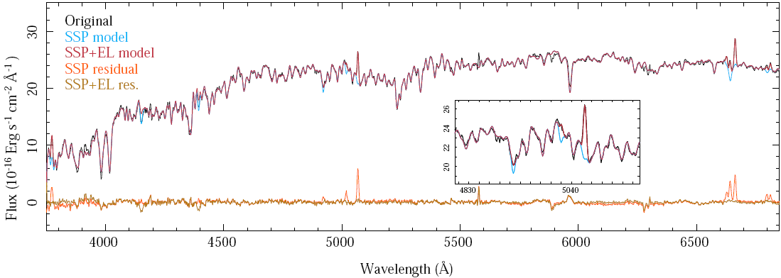
Fig. 3 Results of the SSP and emission line fitting procedure using FIT3D for the central spectrum of NGC 2916 extracted from the V500 datacube of the CALIFA survey, shown in Fig. 2. The black line shows the original spectrum, along with the best fitted stellar population (light blue), and the best fitted combination of stellar population and emission lines (red). Finally the pure emission line spectrum, after subtracting the best model for the stellar population, is shown as a solid orange line, and the residual of the subtraction of the best fitted model including both the stellar population and the emission line model is shown as a light green line. The inset shows the same spectra for the wavelength range between Hβ and O , to highlight the quality of the fitting. The color figure can be viewed online.
3.3. Spatial binning
The central spectra described in the previous section have, in general, a S/N well above 50 for most of the galaxies included in the IFU surveys of our interest (e.g. Sánchez et al. 2012; Bundy et al. 2015). Therefore, they are above the S/N threshold for which the simulations from Paper I (§ 3 and Table 1) suggest that the properties of the stellar populations are well recovered (i.e., within an error of ≈0.1 dex). However, as the surface-brightness of the galaxies declines as a function of the galactocentric distance, the S/N decreases rapidly in the outer regions (e.g., Figure 13, Sánchez et al. 2012), and therefore the results from any analysis of the stellar continuum become unreliable, as already noticed by several authors (e.g. Cappellari & Copin 2003; Cid Fernandes etal. 2013,2014).

In order to overcome this problem a binning scheme is frequently adopted to aggregate spaxels in the outer regions so as to increase the signal to noise ratio. This is a mathematical problem that goes beyond the field of integral field spectroscopy, although it is broadly addressed in this field. A set of solutions has been proposed on the basis of different assumptions and goals, in addition to the main one, i.e., to increase the S/N ratio preserving as much as possible the spectroscopic properties of the data.
One of the simplest methods was proposed by Samet (1984), the so called Quadtree algorithm. This method consists of a recursive partition of the FoV into axis-aligned squares. The initial square corresponds to the entire FoV. Then the FoV is divided in four areas of equal size. Subsequently each of the sub-squares is equally divided. If a certain goal S/N, required as input to the algorithm, is not achieved in the next iteration, then the procedure stops for a particular square. However, if it is achieved, the procedure continues until the original pixel (spaxel) size is reached. This algorithm is extensively explored in Cappellari & Copin (2003). The two main problems of this procedure are that (1) it depends on the actual orientation of the FoV with respect to the original geometry of the galaxies, (2) for the dataset discussed here, with an intrinsic non-square (or rectangular shape), the method should be adapted, and (3) it does not preserve the shape of the original astronomical object.
An alternative method is the isophotal segmentation, first introduced by Papaderos et al. (2002), and implemented for IFU data in Papaderos et al. (2013), and Gomes et al. (submitted). The algorithm segments the FoV on the basis of a set of isophotes, according to the surface brightness distribution. Then each isophotal area is divided in subsequent bins by aggregating adjacent pixels (spaxels) along the azimuthal angle in order to achieve a goal S/N. Therefore, the area of the final spatial bins grows with galactocentric distance (as the surface brightness decreases). The main problem with this approach is that the resulting segmentation/binning depends strongly on some arbitrary parameters, like the number and range of surface brightness of the original isophotes, and the original pixel (spaxel) selected to start the aggregation in each isophote, irrespectively of the goal S/N.
The most broadly used binning scheme for IFS data is the Voronoi binning procedure (Cappellari & Copin 2003). This algorithm was developed to satisfy three requirements, in addition to the main goal of the algorithms described above: (i) the bins should properly tessellate the FoV (i.e., there should be no holes or overlapping areas), (ii) the bin shape has to be as compact or round as possible, and (iii) the scatter of the S/N after the binning should be as small as possible. Under this basic assumption the authors developed an algorithm in which, starting from a set of points within the FoV (called generators), a tessellation based on the Voronoi algorithm is generated. This guarantees that all pixels (spaxels) in a certain spatial bin are the nearest ones to the point that has generated the considered bin. The generators are selected on the basis of a ranking order S/N of the pixels and a distance criterion (Cappellari & Copin 2003).
By construction, this algorithm guarantees a very homogeneous distribution of the S/N; this has made it very popular among the community. However, it does not preserve the original shape of the astronomical object, in particular for galaxies with sharp structures. Furthermore, since the aggregation is based mostly on a S/N criteria, it may include spaxels corresponding to areas of the galaxy with very different physical properties (like spiral arms and inter-arm regions). This issue was never a concern when the algorithm was created, since it was developed under the umbrella of the SAURON project (Bacon et al. 2001), whose main (initial) goal was to explore the central regions of a sample of early type galaxies, and mostly focused on the study of their kinematical properties. The light distribution of an early type galaxy is expected to follow a smooth shape, and the kinematics shows no abrupt changes. Therefore, imposing further criteria to force the spatial bins to follow the shape of the light (like the isophotal method), was not needed. For similar reasons it was broadly adopted in the analysis of the Atlas3D data (Cappellari et al. 2010), and subsequently used in hundreds of studies.
An additional issue regarding the Voronoi binning algorithm is that it assumes that the S/N follows the light distribution. In general, this is the case for datasets acquired with IFUs that cover the complete FoV, like the lens array systems of SAURON (Bacon et al. 2001). In those cases, when the noise budget is dominated by the intrinsic Poissonian noise due to light coming from the astronomical target, the S/N is a function of the surface brightness. For the SAURON and Altas3D data this was the case for most of the targets, since the FoV of the instrument rarely covered more than ≈1.5 effective radius. Thus the noise produced by the sky subtraction and other electronic effects of the detectors were negligible.
However, most of the current IFU surveys adopt a different IFU technology (fiber bundle with an incomplete coverage of the FoV), and the targets are sampled up to 2.5 effective radii and beyond (e.g. Walcher et al. 2014). As a consequence, these basic assumptions do not hold. First, because they use fiber bundles current IFU surveys adopt a dithering scheme in order to cover the complete FoV. In most cases this approach creates an intrinsic in-homogeneous distribution of the S/N, even for exposures of totally flat targets. In the case of the three pointing dithering pattern the spaxels can be covered by one, two, or even three fibers. Therefore, there could be a factor
The published version of the Voronoi binning does not take into account the covariance between adjacent spaxels that is inherent to the image reconstruction schemes required to obtain a datacube from a dithering observation using a fiber bundle. It is known that by co-adding N adjacent spectra the noise does decrease following a
In P 3D we depart from the widely used Voronoi binning scheme and we propose a different algorithm, based on both a continuity criterion for the surface brightness and a goal for the signal-to-noise ratio (Continuum plus S/N binning, CS-binning hereafter). Like the Voronoi binning, CS-binning requires as input a signal-map, a noise-map, and a S/N goal. In addition, in order to be aggregated it requires the difference of fraction of flux between a given spaxel and an adjacent one. In principle, the algorithm looks initially for all the spaxels/pixel for which the S/N is already above the minimum S/N required. Those are selected as spatial bins with a single pixel. Then, for the remaining pixels the algorithm looks for the one with the higher intensity. This will be the seed of the next spatial bin. It derives the S/N at this location and estimates the maximum number of adjacent pixels required to increase that S/N to the target S/N, assuming that adjacent pixels have similar S/N levels. It assumes Poissonian statistics plus the effect of the covariance, and solves for N (the number of adjacent pixels to co-add) from the equation:
 1
1
where S/N input is the estimated signal-to-noise if the noise distribution were Poissonian (i.e., no covariance between adjacent spaxels), N is the number of adjacent spaxels included in a particular spatial bin, and covar(N) is the correction introduced by the correlation of the noise between adjacent spaxels. This last parameter is derived statistically in an empirical way as described in Husemann et al. (2013) and more recently in García-Benito et al. (2015), by creating spatial bins of arbitary size, coadding N adjacent spaxels, computing S/N input and measuring the real S/N from the coadded spectra. Then a functional form for the dependence of covar(N) with the number of coadded spaxels is derived as shown in Figure 11 of García-Benito et al. (2015).
Then, N is used to estimate the radius of the circular aperture required to be integrated to enclose this number of spaxels/pixels:
 2
2
Finally, the algorithm aggregates all adjacent pixels within a maximum distance of R max and for which the flux intensity is within the predefined fraction to the initial seed. In general this creates spatial bins that are not round, since they tend to follow the shape of the isophotes across the FoV Due to the second criterion, in general the S/N goal is not reached for most of the spatial bins. This segmentation/binning scheme is a mix between the isophotal and the Voronoi binning schemes.
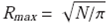
Figure 4 shows a comparison between the adopted CS-binning and the Vorononi binning schemes for the V500 setup data extracted from the CALIFA dataset for NGC 2916. The signal and noise maps adopted for both procedures were created by deriving the median and standard deviation of the flux intensity in each spaxel for the spectral pixels within the wavelength range 5590-5680 Å. In the case of the Voronoi binning it is used only the S/N map. For the CS-binning the signal map is used for the continuity criterion. For both procedures the results depend greatly on the wavelength regime adopted to perform the spatial binning. The Voronoi binning was modified to take into account the spatial co-variance between the data. It shows the distribution of spatial bins when a S/N goal of 40 is selected for the Voronoi binning, and a S/N goal of 50 and a fractional flux variation of 20% between adjacent pixels are accepted for the CS-binning. To allow a fair comparison, the values were selected to reach a S/N>30 in most of the FoV and to have a similar number of spatial bins when using both algorithms (391 in the case of the Voronoi and 439 in the case of the CS-binning).
Fig. 4 Top-left panel: Narrow-band intensity map derived by summing the fluxes within the wavelength range 5590-5680 Å for the CALIFA V500-datacube of NGC 2916. Top-central panel: Segmentation map derived for the same datacube using a continuum plus S/N binning scheme, as outlined in the text. Top-right panel: Segmentation map derived for the same datacube using the most frequently used S/N voronoi binning scheme. Bottom-left panel: Radial distribution of the signal-to-noise for the original datacube (blue squares), the segmented cube based on Voronoi binning (orange stars), and the continuum plus S/N segmented cube (black circles), for the same datacube. Bottom-central panel: S/N map for each of the spatial bins created using a continuum plus S/N binning scheme (the one on the top-central panel), for the same datacube. Bottom-right panel: S/N map for each of the spatial-bins created using a S/N voronoi binning scheme (the one on the top-right panel), for the same datacube. In all the maps the contours are the same as the ones presented in Figure 1, left-panel. The color figure can be viewed online.
As expected, both algorithms create similar single pixel spatial bins for those pixels already fulfilling the S/N critérium. For pixels below the S/N goal the less restrictive Voronoi binning creates larger spatial bins, in particular in the outer regions of the galaxy. We include in the figure the spatial distribution of S/N for both algorithms after applying the spatial binning. By construc tion, the distribution is very homogeneous in the case of the Voronoi binning ({S/N} = 38.5 ± 4.7), and presents a clear structure with a larger dispersion in the case of the CS-binning ({S/N} = 30.7 ± 16.3). The bottom-left panel of Figure 4 shows the radial distribution of S/N for the original dataset and for the two binning schemes. Up to ≈10" the three distributions are very similar (the re gions where no binning is needed). At larger galacto-centric distances the distribution for the Voronoi binning becomes almost flat, as expected from the results presented by Cappellari & Copin (2003). In contrast, the CS-binning provides a S/N ≈40, between 10" and 30", covering a wide range of S/N values (between ≈30 and ≈60). The average S/N in this regime is very similar (but with twice the scatter) to the one provided by the Voronoi binning.
Beyond this distance, the CS-binning gives little improvement in S/N with respect to the original data. However, at those galactocentric distances the original data have S/N<3 in most cases, and we regard those areas useless for the analysis of the underlying stellar population. If we try to reach a S/N above ≈30 by co-adding individual spaxels with a S/N below 3 the area required to be covered by the spatial bin would be so large that the spectra would lose the coherence in their basic properties, as indicated above. Therefore, although it may be mathematically correct the interpretation of the physical properties derived will be always a problem.
This example does not demonstrate the superiority of any of these methods, as this was never our intention. If the goal is to normalize the S/N across the FoV of the data, definitely, Voronoi binning is (so far) the best algorithm. However, for increasnig the S/N preserving the shape of the original target, the CS-binning presents significant advantages. For the current implementation of P 3D we adopted a S/N goal of 50 and a more restrictive upper limit to the range of relative fluxes between adjacent spaxels to be coadded, setting it to a value of 10%, prioritizing to keep as much as possible the original shape of the data rather than the final S/N of the spectra. By increasing the fractional flux variation one can achieve a S/N closer to the goal, with the correspond ing loss of spatial information. If no limit is imposed to the fractional flux variation, the binning provided by both methods is very similar.
The procedure provides a S/N map before and after binning, and a segmentation map in which each pixel corresponding to the same spatial bin is labeled with the running index that identifies the spatial bin. All those maps are stored as FITS format files.
3.4. Analysis of the stellar population
As described above, the original cube is spatially binned using the CS-binning algorithm. The spectra corresponding to the spaxels within each spatial bin are averaged and stored as a single spectrum, together with the average spatial coordinates. Thus, for each bin we obtain a spectrum that corresponds to the mean of each individual spectrum of all the spaxels within that spatial bin, masking spectral pixels with bad values. At the end of this process, a row stacked spectrum (RSS) is created and a position table for each binned cube, following the order of the spatial bin indices (from the brightest to the faintest areas in the cube, by construction). In addition an intensity map at the wavelength range corresponding to the F-band before and after performing the binning is provided. The ratio between both maps is the relative contribution of each pixel to the average intensity within the spatial bin where it is aggregated. This ratio will be used later in the dezonification process, which will be explained below (Cid Fernandes et al. 2013).
Each spectrum within the RSS file is analyzed following the same procedures applied to the central spectrum, as described in § 3.2.1. The goals of this analysis are the following: (i) to obtain the best representation of the underlying stellar population to subtract it from the original data and provide a spectrum of the emission lines (pure emission line spectrum); (ii) to characterize the main properties of the underlying stellar population, as described in Paper I, § 2.3.
Following the procedures discussed, the stellar continuum is first fitted with a simple template of SSPs in order to derive the systemic velocity, velocity dispersion, and dust attenuation (miles12). Then the main properties of the strong emission lines are derived by fitting the residual spectrum (after the underlying stellar population is subtracted) with a set of Gaussian functions. This first model of the emission lines is subtracted from the original spectrum to remove the effects of the strongest emission lines. Finally, this spectrum is fitted with the gsd156 template library, defined in § 3.2.1, to derive the main properties of the stellar populations (age, metallicity, star-formation history, etc). As described in Paper I, § 2.2, the procedure may be iterated until it fulfills a certain convergence criterion (i.e., until the X 2 decreases to less than a certain percent). In this particular implementation we iterated just 2 times, to speed up the process and because of the limited improvement in terms of the X 2 between sucessive iterations.
The main differences with respect to the procedure described in § 3.2.1 and Paper I, § 2, are:
• The velocity dispersion (σ) for the first spectrum, that corresponds to the peak intensity of the galaxy, and therefore to the central region, is explored within a wide range of values up to 400 km/s (in addition to the instrumental dispersion that is first applied to convolve the SSP template). Then, for successive spectra, corresponding to spatial bins of lower flux intensity, the exploration of the velocity dispersion is restricted to a range between 0.5 and 1.5 times the value of the previous iteration, i.e., 0.5σi < σ i+ 1 <1.5 σi, where i is the index of the spatial bin.
This procedure ensures that the velocity dispersion is kept within reasonable values for areas of lower S/N (lower intensity, i.e., in the outer part of the galaxies). It is known that at lower S/N all fitting procedures tend to increase the velocity dispersion to fit the average distribution of values that is dominated by the noise.
• In the case of MaNGA data, the procedure is repeated twice, using a different template in the first step, due to the wider wavelength range covered by MaNGA. First, we adopted a template adopted extracted from the MIUSCAT SSP library (Vazdekis et al. 2012). This library is an extension of MILES, covering the wavelength range 3465-9469 Å, with a similar spectral resolution and spectrophotometric quality. We adopted a grid of MIUSCAT SSPs including four stellar ages (0.06, 0.20, 2.00, and 17.78 Gyr), and three metallicities (0.0004, 0.02, and 0.0331), subsolar, solar, or supersolar. For this particular library we include ages slightly younger than the ones included in miles12, since we have seen that they tend to reproduce slightly better the blue end of the MaNGA spectra (not covered by CALIFA and SAMI). The results of this first analysis are used only to characterize the underlying stellar population in the wider possible wavelength range, and to provide the best emission line spectrum (i.e., the orange spectrum in Figure 3). This would provide a GAS-pure cube over almost the complete wavelength range covered by MaNGA. The results are also used to derive the non-linear parameters of the stellar populations (velocity, velocity dispersion and dust attenuation)
In the second step the same parameters are used, wavelength ranges, stellar templates, and initial guess values for the three surveys (CALIFA, MaNGA, and SAMI), in order to homogenize the results as much as possible. However, to speed-up the processes, in the case of MaNGA we do not repeat the derivation of the non-linear parameters of the stellar populations, but use the result from the first step described before.
• For MUSE data (e.g. Sánchez et al. 2015 a) the same stellar templates and guess parameters were adopted as for MaNGA, but restricting the wavelength range to that of MUSE. Since for low-z objects MUSE does not cover the 4000Å break, we are still not sure about the accuracy of the parameters derived for the stellar populations, which should be compared with ad hoc simulations, similar to the ones shown in Paper I, § 3.2.
The analysis of the stellar populations performed using FIT3D on the RSS file provides three different data-products, two csv files, and a FITS format cube:
The first of the two csv files, named auto_ssp.CS.OBJECT.rss.out, is an ascii table. Each row comprises the main properties of the stellar population derived by the fitting procedure for each individual spectrum within the RSS file (and therefore each spatial bin within the binned cube). The parameters distributed in each column include the reduced X 2 of the fit, the luminosity -and mass-weighted log-ages and log-metallicities of the stellar populations, as defined in Paper I, § 2.3. In addition it contains the dust attenuation, the systemic velocity, and the velocity dispersion, with their corresponding errors. It also includes the average intensity and standard deviation of the residuals from the fitting procedure, and the average mass-to-light ratio within the spatial bin.
The second csv file, named coeffs_auto_ssp.CS. OBJECT, rss. out, is a table with one row for each SSP in the library and for each spectrum in the RSS file (i.e., number of spatial bins). The columns include a running index corresponding to the SSP, age, metallicity, and mass-to-light ratio of this population, along with the fraction of light that it contributes to the original spectrum at the normalization wavelength with its estimated error. This information is used to derive the luminosity- and mass-weighted parameters included in the first file.
Finally a FITS format cube, named output.auto_ssp. CS.OBJECT.rss.out.fits. gz stores the original spectra, the best model spectra, pure emission line spectra, the residuals from the fit of the emission lines (as indicated below), and the spectra after subtracting the best model for the emission lines. In this FITS format cube each slice along the Z-axis comprises the results from the fitting procedure for each spectrum in the RSS file.
The derived dataproducts included in the two csv files are rearranged into a set of maps (one for each dataproduct), following the original spatial shape of the datacubes, by associating each value to the location in the 2D space defined by the segmentation file, as described in § 3.3. This format is convenient to store and share the data, to compare different dataproducts, and for plotting purposes. The maps of these dataproducts are stored in separate FITS format files, named map. CS. OB J_PARAM_ssp. f its. gz, where OBJ is the object name (as it appears in the name of the datacube) and PARAM is a label indicating each of the derived dataproducts. For example, the FITS file map.CS.NGC2916_age_ssp.fits.gz stores the luminosity-weighted age derived for the CALIFA V500 datacube of NGC 2916. All the files generated by P 3D for the V500 datacube of NGC 2916 described in this section can be found in the FTP15. In § 3.7 we provide the correspondence of each FITS file with the measured parameter, for the distributed dataproducts.
3.4.1. Stellar Kinematics
Figures 5 and 6 illustrate the results of the kinematics analysis for the stellar populations. The figures show that the estimated velocities agree within ±30 km/s across the entire FoV of the three datasets. For the velocity dispersion, the three datasets agree just within the central ≈8", as expected from the simulations presented in Paper I (e.g., Table 1 of that paper). The V500 and V1200 datasets of the CALIFA survey agree up to to distances ≈10". Beyond that galactocentric distance, the velocity dispersion derived for the V1200 data collapses to the minimum selected value of 20 km/s, fixed in the presented version of P 3D at the limit of what is feasible at the resolution of the data. This indicates that we should re-analyze all the datasets allowing the ex ploration of lower velocity dispersion values. For the V500 dataset we have applied an overall quadratic offset of 120 km/s to match the velocity dispersion; this indicates that the offset between the SSP resolution and the instrumental resolution should be revised and that in the current analysis we have a miss-match of ≈30% in the assumed instrumental resolution for the V500 data. This offset does not affect the derivation of the properties of the stellar populations, since the final velocity profiles are well constrained, being affected only the derivation of the velocity dispersions. The offset was derived from the comparison of the peak velocity dispersion at the cen ter of the galaxies, obtained by the pipeline for the ≈500 objects in common between the two CALIFA setups. After this correction the velocity dispersion for the V500 dataset presented a cut at ≈10", a location at which the values derived were dominated by the instrumental resolution. For the P-MaNGA dataset the velocity dispersion measured beyond 9" presented a large dispersion, with an offset with respect to the values derived using both the V1200 and V500 CALIFA datasets. We still do not know the origin of this discrepancy , although most probably it comes from the fact that the P-MaNGA data were taking during an experimental phase of this project, using dif ferent fibers and packing, which may alter the nominal spectral resolution.
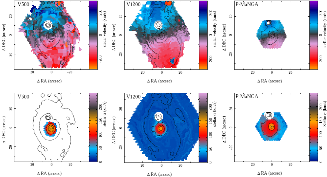
Fig. 5 Stellar velocity (top panels) and velocity dispersion maps (bottom panels) derived using the three datasets for NGC2916: left CALIFA V500 setup; central CALIFA V1200 setup; right. P-MaNGA dataset. For the velocity dispersion the values below the instrumental velocity dispersion have been masked. The color figure can be viewed online.
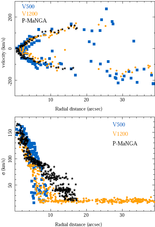
Fig. 6 Stellar velocity along a pseudo-slit located at the center of the galaxy and tilted 60° (top panel), and radial distribution of the velocity dispersion (bottom panel) extracted from the kinematic maps of the galaxy NGC2916 shown in Figure 5 for the three datasets: CALIFA V500 setup (blue squares), CALIFA V1200 setup (orange circles), and P-MaNGA (black stars). The color figure can be viewed online.
3.4.2. Composition of the stellar population
Figures 7 and 8 illustrate the results from the analysis of the properties of the stellar populations. Both figures show the 2D and radial distributions of the luminosity-weighted log-age and log-metallicity, the surface mass density, and the mass-to-light ratio for the three different datasets. The log-ages agree within a range of ±0.2 dex, for the central regions (<15״) of the three datasets, as expected from the simulations presented in Paper I (e.g., Table 1 of that paper). At larger radii, we are not able to compare with the P-MaNGA results (due to the smaller FoV of this dataset). However, the analysis performed over the V1200 data seems to result in slightly higher log-ages (≈0.2 dex) than the ones derived from the V500 one. On average, an inaccuracy/offset of ≈0.1 dex is found between the derived log-ages using the CALIFA V500 and both the V1200 and P-MaNGA dataset, with a dispersion of σ ≈ 0.1 dex. Between the V1200 and the P-MaNGA data there is very good agreement, with an offset of 0.03 dex and a dispersion of σ = 0.06 dex.
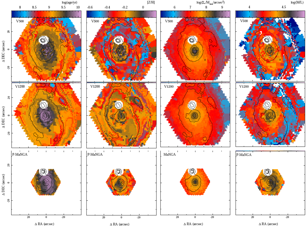
Fig. 7 From left to right, distribution of the luminosity weighted age and metallicity, mass surface density, and mass-to-light ratio of the stellar population in NGC 2916 across the FoV for the three datasets. Top panels: CALIFA V500 setup. Central panels: CALIFA V1200 setup. Bottom-right. P-MaNGA dataset. Contours correspond to the same intensity level of the broad band images presented in Figure 1. The white masked region north-east of the center of the galaxy corresponds to a foreground star, visible in Figure 1. The color figure can be viewed online.
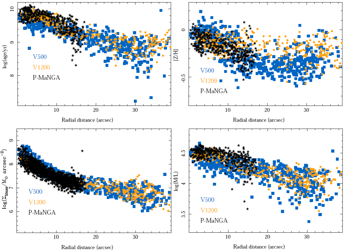
Fig. 8 Radial distribution of the luminosity-weighted age (top-left panel), metallicity (top-right panel), mass surface density (bottom-left panel), and mass-to-light ratio (bottom-right panel) of NGC 2916 also shown in Figure 7 for the three datasets: CALIFA V500 setup (blue squares), CALIFA V1200 setup (orange circles), and P-MaNGA (black stars). The color figure can be viewed online.
For the stellar metallicity we found agreement within a range of ±0.1 dex for the three datasets in the shared FoV, although in the inner regions the values derived for the V1200 are slighly smaller. This is consistent with the larger values derived for the ages and the well-known age-metallicity degeneracy. For larger radii the derivation based on V1200 data seem to present a slightly larger log-metallicity (≈0.1 dex). Indeed, the agreement between the results derived using the CALIFA V500 dataset and the P-MaNGA ones is remarkably good, with an offset of -0.02 dex and a dispersion of 0.06 dex. Taking into account the limited wavelength range of the CALIFA V1200 data compared to the other two datasets (e.g., Figure 2), a range that does not cover those features more sensitive to the variation of metallicities, like the Fe and Mg absorption features between 5100-5400Å, this result is somehow expected. This range does not cover the stronger spectral features sensitive to the analyzed parameters, and the wavelength range is too short to be sensitive to the dust attenuation.
For the regions covered by the three datasets the surface mass density shows very good agreement, within the range of the dispersion of each individual dataset. The agreement is better between the two CALIFA datasets than between them and the P-MaNGA data, with an offset of -0.01 dex and a dispersion of 0.12 dex, in the first case, compared with an offset of ≈-0.1 dex and a dispersion of 0.1 dex, in the second case. In both cases the dispersion is consistent with the limit in the accuracy of the mass estimation found by different authors using this methodology (González Delgado et al. 2014, e.g). The offset is most probably due to the different spectrophotometric calibration adopted in each survey (García-Benito et al. 2015; Yan et al. 2016), explaining why the two CALIFA datasets present a better agreement.
Finally, the mass-to-light ratio presents a similar distribution for the three datasets at different galactocentric distances, although there seems to be a systematic offset between the three estimations. Like in the case of the stellar mass density, the offset is larger for the CALIFA datasets compared to the P-MaNGA ones (0.07-0.10±0.04-0.06 dex), than among the former two (0.03±0.05 dex).
All these Figures confirm the consistency of the results for the stellar population analysis obtained by PIPE3D based on different datasets with differences within the expected range, based on simulations (Paper I, Table 1), and they are also consistent with previous results (e.g. Cid Fernandes et al. 2013; González Delgado et al. 2014).
3.4.3. Emission lines in the binned data
As explained in Paper I (§ 2.4) and briefly described in § 3.4, FIT3D fits the emission lines in a quasi-simultaneous way with the stellar populations, adopting an iterative scheme. According to this, the residuals from the analysis of the stellar population are fitted with a set of Gaussian functions to characterize the properties of the emission lines, and the best model of the emission lines is subtracted from the original spectra to perform the analysis of the stellar population in a second iteration.
This iterative scheme was adopted for the analysis of the RSS file provided by the CS-binning. In the current implementation of P 3D we included in the analysis loop the fitting to a set of strong emission lines frequently observed in the optical range of galaxies: [O ]λ3727, Hδ, Hγ, Hβ, [O ]λ4959, [O ]λ5007, [N ]λ6548, [N ]λ6583, Hα, [S ]λ6717, and [S ]λ6731. Each of these emission lines was fitted with a single Gaussian profile for the pure emission line spectrum at each spatial bin derived from the analysis of the stellar population.
The final product of this fitting procedure is an table named elines_auto_ssp.CS.OBJ .rss.out that comprises, for each spectrum in the CS-file and for each emission line, a set of columns including: (1) the nominal wavelength of the emission line, (2) its integrated flux, (3) the σ (dispersion in Å) of the Gaussian fitted, and (4) the systemic velocity with the corresponding uncertainties estimated by FIT3D. As in the case of the stellar population, all dataproducts are rearranged into a set of maps, following the original spatial shape of the datacubes, by associating the given value to the location in the 2D space, defined by the segmentation file described in § 3.3. In a way similar to the analysis of the stellar populations, the parameters derived for each emission line are stored in separate FITS format files, named map. CS. OB J _PARAM_WAVELENGTH. fits. gz, where OBJ is the object name (as it appears in the name of the datacube), PARAM is a label that identifies each of the dataproducts, and WAVELENGTH is the nominal wavelength of the emission line. For example, the FITS file map.CS.NGC2916_flux_6562.fits.gz stores the flux density of Hα derived from the CS-binned RSS file extracted from the CALIFA V500 datacube of NGC 2916. As indicated above, all the files generated by P 3D for the V500 datacube of NGC 2916 can be found in the FTP indicated above.
Figure 9 illustrates the result of this analysis, showing the Hα flux intensity and velocity maps for the CS-binned data, after being rearranged into the original spatial shape of the datacubes. In both panels it is possible to clearly identify the original CS segmentation. This segmentation was created on the basis of the flux intensity and S/N of the continuum, and in general, does not reproduce the corresponding parameters for the emission lines. It does not only degrade unnecessarily the spatial resolution of the emission line maps, but also it can blur the signature of weak emission lines by co-adding in the same spatial bin emission lines with different kinematics, and it may also significantly affect the estimated equivalent width. This effect can be clearly observed in the velocity maps of the areas displaying weak emission.
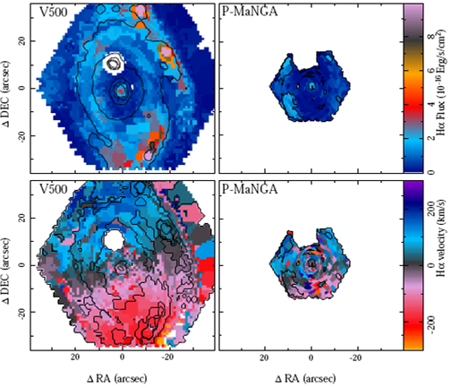
Fig. 9 Hα intensity and velocity maps (top and bottom panels respectively) derived using the CS-binned RSS files obtained from the CALIFA V500 (left panels) and the MaNGA (right panel) datasets of NGC 2916. In the left-hand panels contours correspond to the same intensity level of the broad band images presented in Figure 1. In the right-hand panels contours correspond to the Hα intensity maps shown in the left-panels, starting at 0.05 10-16 erg s־1 cm-2 arcsec-2 with a constant step of 1 x 10-16 erg s־1 cm-2 arcsec-2. The color figure can be viewed online.
3.4.4. Dezonification
The dezonification procedure was first presented by Cid Fernandes et al. (2013) in order to provide an accurate estimation of the spatial distribution of the stellar properties. In P 3D we use it to decouple the analysis of the emission lines from the spatial binning required to perform an accurate analysis of the stellar continuum. This procedure takes into account the relative contribution of each spaxel to the spatial bin in which it is aggregated, as explained in § 3.4. This is the so-called dezonification map.
The procedure is done performing the following steps:
An empty datacube is created with the same spatial and spectral shape as the original cube. The result of the dezonification procedure will be stored in this datacube.
As indicated before (§ 3.4 and 3.4.3), for each cube a CS-binning was performed, extracting a RSS-file that was fitted with a SSP stellar library (plus emission lines). This provides a multi-SSP model for each spatial bin.
For all the spaxels within the same spatial bin the same multi-SSP model is adopted, which is stored in the empty datacube described before at the corresponding spatial coordinates of each spaxel.
Repeating this procedure for all the spatial bins, we end up with a datacube where the SSP-model corresponding to each spaxel is stored. However, in this datacube the spectra corresponding to the spaxels within the same spatial bin are all the same, keeping the spatial shape of the CS-segmentation.
This preliminary model datacube is multiplied by the dezonification map to match the flux intensity of each spectral model with that of the original cube, spaxel-by-spaxel. The dezonification map, explained in § 3.4, is the ratio between the broad-band intensity maps of the original and CS-segmented datacubes. Thus, it is the relative contribution of each spaxel to the intensity in the corresponding spatial bin.
Then, in order to take into account the mismatch between adjacent spectra corresponding to different spatial bins, the new cube is smoothed spatially with a Gaussian kernel having the size of the expected PSF of the datacubes (≈2.5"-3"), preserving the flux intensity in each spatial resolution element.
The product of this procedure is a cube comprising a model of the underlying stellar population with a continous spectral shape and adjusted to the flux intensity of the original cube. This cube is stored in a FITS format file named SSP_mod.OBJ.cube.fits.gz.
Finally, this cube is subtracted from the original one providing a set of spectra that include only the emission lines from the ionized gas and the residuals from the analysis of the stellar population. A low order polynomial is fitted to the continuum of this residual cube in order to remove inaccuracies in the spectrophotometric calibration, or template mis matches (e.g. Husemann et al. 2013; Cid Fernandes etal. 2013; García-Benito etal. 2015).
The final product of this analysis is the so called pure emission line cube, and it is stored in a FITS format file named GAS. OB J . cube. f its. gz.
3.5. Analysis of the strong emission lines
An analysis of the emission lines using the pure emission line cube is implemented in order to derive the properties of the ionized gas with the best spatial resolution, and independently of the S/N required to analyze the continuum. The strongest emission lines in the wavelength range studied (from the list described in § 3.4.3) are fitted with a single Gaussian function. This parametrization, implemented in the current version of P 3D is valid for most of the emission lines observed over a large fraction of the optical extension of the galaxies. However, this approach is too simplistic in some cases (e.g., gas rich major mergers, overlapping foreground galaxies, or cores of AGNs). In future versions of the pipeline we will implement a multi-component analysis (already foreseen in FIT3D). The only limitation of this approach is the that the analysis will be more time consuming.
The emission lines are grouped into four groups that are considered to be kinematically coupled (for simplicity). Each group is fitted within a wavelength range, adjusted to the observed frame on the basis of the galaxy redshift. The four groups include the following emission lines and rest frame wavelength ranges: (i) [O ]λ3727 (3700-3750); (ii) Hβ, [O ] λ4959, and [O ] λ5007 (4800-5050); (iii) [N ] λ6548, Hα, and [N ] λ6583 (6530-6630); and [S ]λ6717 and [S ]λ6731 (6680-6770). Before any of these lines is fitted with a single Gaussian, a first guess for the kinematics is done on the basis of the expected Hα wavelength at the galaxy red-shift and by performing a parabolic approximation to the centroid of the emission line. This procedure is broadly used in the detection of peak intensity fluxes, like in the case of the reduction of fiber fed spectrographs, being fast and very reliable (e.g. Sánchez 2006 a). Then the emission lines are fitted using a narrow range of systemic velocities centered on the initial guess, and limiting their width to the nominal instrumental dispersion.
The result of this analysis is a set of maps with the spatial shape of the pure emission line cube, which includes the various parameters derived for each emission line as described in § 3.4.3. These maps are stored in a set of FITS format files, named map. W1_W2 . OBJ_PARAM_NN.fits.gz, where OBJ is the galaxy name (as it appears in the name of the dat-acube), PARAM is a label indicating each of the derived dataproducts, W1 and W2 are the wavelength ranges of each emission line group, as described above, and NN is an index indicating the order of the emission line within each group. For example, the FITS file map. 6530.6630. NGC2916_flux_00.fits.gz stores the flux density of Hα obtained from the pure emission line cube derived for CALIFA V500 data of NGC 2916. The emission line fluxes are not corrected for extinction. This should be accomplished by the usual procedures, e.g. analyzing the Balmer line ratios, as we will describe in § 4. Like in the previous cases, an example of these files is stored in the FTP indicated above and described in § 3.7.
Figure 10 illustrates the result of this analysis, showing the Hα flux intensity and velocity maps derived from the pure emission line cube. On the other hand, Figure 9 highlights the differences between the parameters derived when the analysis of the emission lines is, or is not, coupled with the spatial binning required to analyze the stellar population. As anticipated, the emission lines are blurred in those areas where the continuum intensity is lower, and therefore larger spatial bins are required to achieve a sufficient S/N. In some cases the gas kinematics is also clearly affected. The effect is stronger in the P-MaNGA data than in the CALIFA ones, due to the lower S/N of the former. The final MaNGA observing strategy (Law et al. 2015), with a minimum goal for the S/N, guarantees that this will not be the case for the final dataset. However, for the P-MaNGA data a fixed exposure time was selected, which has a larger effect on the continuum S/N at this spectral resolution.
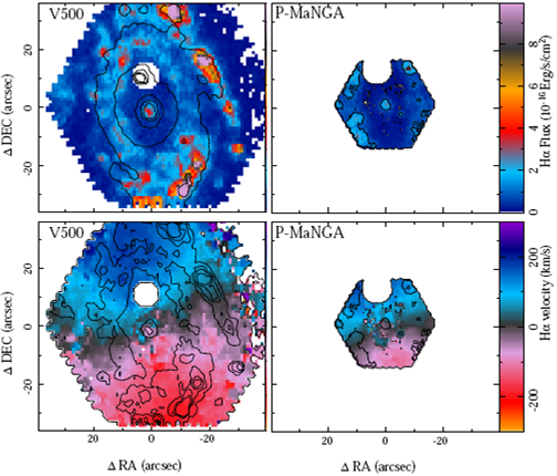
Fig. 10 Hα intensity and velocity maps (top and bottom panels respectively) derived using the emission line pure cubes obtained from the CALIFA V500 (left panels) and the P-MaNGA (right panel) datasets of NGC 2916. In the left-hand panels contours correspond to the same intensity level of the broad band images presented in Figure 1. In the bottom panels the contours correspond to the Hα intensity maps shown in the left-panels, starting at 0.05 10-16 erg s־1 cm-2 arcsec-2 with a constant step of 1 x l0-16 erg s-1 cm-2 arcsec-2. The parameteres presented in this figure were obtained after dezonification. The color figure can be viewed online.
3.6. Analysis of the weak emission lines
So far we have characterized the strongest and more frequently observed (and studied) emission lines within the wavelength range considered. However, there are many more weak emission lines. Table 1 lists the usual emission lines observed in ionized regions of our Galaxy in the common wavelength range between the three IFU surveys considered here. This list was extracted from those detected in classical H regions, like the Orion nebula (Baldwinetal. 1991; Sánchez et al. 2007 c). Those emission lines that are accessible to MaNGA only due to its larger wavelength coverage are indicated.
It is not practical to perform a Gaussian fit, like the one described in the previous section, for all the ≈50 emission lines and for all the spectra in each datacube, since it is very time consuming. Therefore, we have adopted a different scheme to extract the main properties of these emission lines: flux intensity, velocity and velocity dispersion, and equivalent width.
This procedure is not a Gaussian fit, but rather a direct estimation of these parameters. It requires as input the pure emission line and the stellar population model cubes described in § 3.4 and 3.4.4, together with an error cube provided by the data reduction. In addition, it requires a list of the emission lines to be analyzed, with their corresponding identifications and nominal wavelengths (like in Table 1), and an estimation of the gas velocity (in km/s) and velocity dispersion, including the instrumental dispersion, in Å. The output of the Hα emission analysis described in § 3.5 is adopted for these latter entries.
After reading the required input, the algorithm performs the following steps: (i) For each emission line in the list, and for each spectrum in the pure emission line cube, it estimates the expected observed central wavelength of the emission line taking into account the initial guessed velocity (λ obs). Then a wavelength range is selected within ±FWHM of the emission line, derived from the initial guessed dispersion (σ in): [λobs-2354σin, λobs+2354σin ]; (ii) Within this wavelength range a set of 50 MC realizations of the spectra are performed, by co-adding to the original flux the error noise multiplied by a random number between ±0.5; (iii) For each MC realization (mc), and for each spectral pixel (i) at a wavelength λ i, the extended flux intensity is estimated if the emission line was well characterized by a Gaussian function centered at λ obs with a dispersion σ in, using the formula:
 3
3
where
 4
4
Where:
 5
5
and λ rest
is the rest frame nominal wavelength of the emission line, c is the speed of light, and
(vi) Finally the velocity dispersion (σ) is estimated on the basis of the second order moment of the distribution, for each MC realization. This approach is adopted due to the complexity of solving Equation 3 for this parameter:
 6
6
It is then transformed to FWHM by the scaling factor (FWHM = 2.354σ). The dispersion also includes the instrumental resolution, that should be subtracted quadratically in any further analysis; (vii) In addition, the EW of the corresponding emission line is obtained by dividing the intensity by the flux density of the underlying continuum, derived as the average within two 30Å wide spectral windows centered at ±60Å from λ obs, of the spectrum extracted from the stellar population model (i.e., once the emission lines are subtracted). The band width is large enough to smooth out any significant contribution by most of the stellar absorption features, although some effect is impossible to avoid; (vi) The average and the standard deviation of the four parameters obtained for each MC realization and for each spaxel are derived and stored in a set of 2D arrays with the same spatial shape as the original cube; (viii) The final dataproducts for each emission line comprise eight 2D arrays, four for the parameters derived and four more for the errors. The complete set of 2D arrays for all the emission lines analyzed is stored in a datacube named flux.elines. OBJ . cube. fits. gz, in which each 2D slice corresponds to a particular dataproduct (or its error) for each of the emission lines analyzed. The header comprises a set of keywords named NAMEXX that store the correspondence of the slice XX to a particular emission line and dataproduct. We note once more that emission line fluxes are not corrected for internal extinction in the galaxy.
Figure 11 shows the comparison between the parameters derived using this algorithm and the values derived using the Gaussian fitting procedure for Hα when analyzing the pure emission line cube for the CALIFA V500 dataset. The integrated flux intensity is the parameter that presents the smallest differences between the two procedures (∆F=0.02±0.25 10-16 erg s-1 cm-2). For the velocity the agreement is within the expectated errors (∆vel=9.6±11.7 km/s). The largest relative differences are found for the velocity dispersion, although they lie within the expectations from the estimated errors (∆σ=0.8±0.66 Å, which corresponds to σ vel = 37 ± 31 km/s). No correction is applied based on these differences, since a priori we do not know which of the two results is more accurate. More simulations are required in this regard.
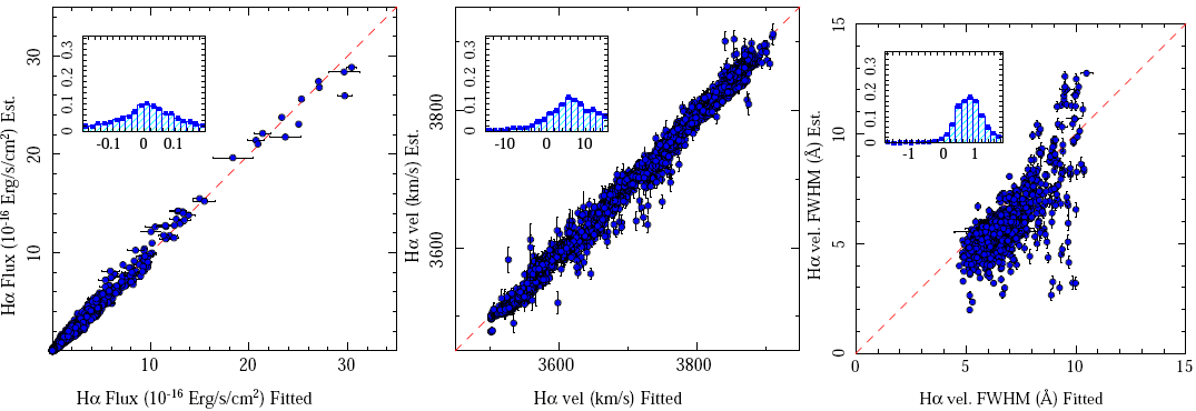
Fig. 11 Comparison between the integrated flux intensity (left panel), velocity (central panel), and velocity dispersion (FWHM, right panel) for the Hα emission line extracted from the pure emission line cubes from the CALIFA V500 based on the Gaussian fits described in § 3.5 (x-axis), versus the values derived using the algorithm described in § 3.6 (y-axis). The error bars indicate the errors estimated by each procedure. For the velocity and velocity dispersion we show only the ≈2700 spaxels for which the Hα flux density is larger than 0.5 10-16 erg s-1 cm-2 arcsec-1. In each panel the inset shows the normalized histogram of the difference between the two estimations. The color figure can be viewed online.
In general, when the emission lines are well de-blended this algorithm produces reliable results. Indeed, based on extensive simulations as described in Paper I (§ 3.3), the accuracy of the recovered parameters is very similar to that estimated for the Gaussian fits. However, it seems that there is a non negligible systematic offset between the kinematic parameters derived from both methods; this should be clarified by simulations. Like in the case of the method described in § 3.5 (assuming a single Gaussian function per emission line), this procedure is not valid to analyze heavily blended emission lines, such as multi-component kinematics and/or broad emission lines due to outflows or AGNs.
The major advantage of this procedure is speed. Using a single core i7 processor it takes about one hour to analyze a single emission line using the Gaussian fitting algorithm described in § 3.5 for a CALIFA-like datacube (or a MaNGA datacube for the bundles with the largest FoVs). In contrast, for the direct estimation procedure it takes ≈3 minutes to analyze the ≈50 emission lines listed in Table 1. Its disadvantage is that it requires a prior estimation of the properties of the gas kinematics. For this reason, in P 3D we first perform a Gaussian fit for a set of strong emission lines and we adopt the new algorithm for a much wider set of weaker (in general) emission lines. We are exploring alternative solutions to speed up the process even more.
3.6.1. Stellar Indices
A classical technique to characterize the properties of the stellar population in galaxies is to measure certain line strength indices, such as the Lick/IDS index system (e.g. Burstein et al. 1984; Faber et al. 1985; Burstein et al. 1986; Gorgas et al. 1993; Worthey 1994). When comparing with the expected values derived using stellar population synthesis models, indices can be used to infer stellar population parameters such as age, metallicity, and a enhancement (e.g. Trager et al. 2000; Gallazzi et al. 2005). They provide robust, model-independent, information, complementary to that provided by fitting the full spectrum with multi-SSP templates, as described in § 3.4. In general, the method employs a combination of indices mostly orthogonal in the physical parameter space (i.e. age and metallicity), like D4000 or Hδ (sensitive to the age), and Mgb or [MgFe]' (sensitive to the metallicity), where [MgFe]' is a combined stellar index, given by the formula:
 7
7
As briefly described in Paper I, § 4, FIT3D includes a script to derive the equivalent widths of a predefined set of stellar indices. The algorithm follows the prescriptions implemented in (Cardiel et al. 2003), slightly modified to take into account the format of the dataset analyzed. It requires as input the output from the previous analysis, described in § 3.4 and § 3.4.3. In particular, it uses the files output.auto_ssp. CS.OBJECT.rss.out.fits.gz and auto_ssp.CS.OBJECT.rss.out, and a number of MC simulations. The algorithm uses the spectrum, after subtracting the strong emission lines for each spatial-bin, and it takes the residuals from the analysis of the stellar population as a hint of the noise pattern, in order to perform a set of MC realizations of the data. Then it estimates the equivalent width for each of the stellar indices using the formula included in for each of the MC realizations. The bandwidths adopted to derive the equivalent width are redshifted to the observed wavelength range using the velocity estimated for each spectrum from the analysis of the stellar population, included in the input files. Finally, the average and the standard deviation for the different values estimated for each MC simulation are derived. These parameters are stored in an ASCII file named indices. CS.OBJ.rss.out, that is later transformed to a datacube named indices.CS.OBJ.cube.fits.gz by associating the value to the location in the 2D space defined by the segmentation file described in § 3.3. This final datacube comprises a set of slices, each one including the value derived for the stellar index (mean value) and its estimated error (standard deviation).
Table 2 shows the list of stellar indices included in the analysis, along with the adopted bandwidths for each index, and the blue and red wavelength ranges from which the continuum is estimated. By construction, these bandwidths were selected to be compatible with (Cardiel et al. 2003), an algorithm that allows the estimatation of the age and metallicity of the stellar population based on a comparison with the expected values of a pair of indices with the corresponding ones of a stellar template, as described in Paper I, § 4. This procedure was already used in the analysis of previous IFU data, as described in Sánchez et al. (2011) and Sánchez et al. (2012).
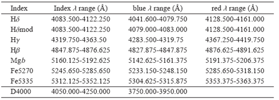
The dependence of the different stellar indices on the age and metallicity of single stellar populations has been explored in detail using SSP models or more complex SFHs (e.g. Poggianti & Barbara 1997). To illustrate how the derived stellar indices compare with the luminosity- weighted ages and metallicities derived from the procedure described in § 3.4 we show a few of them in Figure 12. As expected, there is a clear trend between the stellar indices and the corresponding physical parameter to which they are sensitive. It is also known that those indices are sensitive to other physical parameters. It is beyond the scope of this article to study this effect in detail, since our aim is to show the different dataproducts delivered by Pipe3D. These results will be analyzed in future studies.

3.7. Packing of the dataproducts
P 3D produces a large number of intermediate data-products that are usually stored either as FITS files, corresponding to the maps containing the values and errors of each of the estimated parameters, or as ASCII files, as tables with the different parameters listed either for each spaxel or for each spatial bin. Since the main goal of this pipeline is to produce dataproducts that are easily distributed, shared and compared between different researchers and for different surveys, we have provided a simple solution: (1) All dataproducts are stored in 2D maps following the spatial shape of the original datacubes, and keeping the original WCS; (2) then, those corresponding to a similar kind of analysis are packed together and stored in datacubes with the same spatial shape of the dataproducts (and the original cube), which correspond to a set of maps arbitrarily ordered along the 3rd dimension, with a header keyword (DEC_XX) indicating which parameter is stored in each slice (XX) of the datacube; (3) the dataproducts corresponding to spatial bins are resampled to the original spatial shape without any interpolation, just associating the same value to all the spaxels corresponding to the same spatial bin. The segmentation and dezonification files are stored in order to allow the user to dezonify a particular integrated property and identify in an easy way which spaxels are binned together; (4) A total of three dataproduct cubes, in addition to those already described corresponding to the stellar indices (§ 3.6.1) and the weak emission lines ones (§ 3.6), are delivered comprising: (i) the dataproducts derived from the analysis of the stellar popu lation (OBJ . SSP. cube. fits. gz); (ii) the dataproducts describing the stellar decomposition or star formation history (OBJ.SFH.cube.fits.gz); (iii) the dataproducts describing the properties of the strong emission lines (OBJ.ELINES.cube.fits.gz). Tables 3, 4, 5, and 6 list the descriptions of the different dataproducts stored in each slice for each of the datacubes, as indicated in the header keywords.
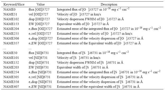


4. A PRACTICAL IMPLEMENTATION OF PIPE3D
Along this article we have described in detail the different procedures implemented in P 3D to characterize the physical properties of the stellar populations and the ionized gas of galaxies observed by the major currently on-going IFU surveys. In this section we present a practical implementation showing the results of applying P 3D to a particular dataset: the 200 cubes that comprise the CALIFA DR2 for the V500 setup (García-Benito etal. 2015)16.
The list of individual objects, including their nominal names and the corresponding CALIFA identifications, together with the coordinates, is given in Appendix B, Table 8 In addition, the table includes some of the main global properties derived by Pipe3D: (i) the redshift, (ii) the stellar mass integrated within the FoV of the datacubes; (ii) the corresponding star formation rate17. We should note that we have co-added all the emission within the FoV irrespectively of the nature of the ionization. Therefore, the SFR listed here should be considered as a linear transformation of the Hα luminosity in a general sense. The errors derived by Pipe 3D have been propagated and included in the table.
Figure 13 shows a comparison of these parameters with those reported in previous studies (Sánchez et al. 2013; Walcher et al. 2014; Catalán-Torrecilla et al. 2015), for the galaxies in common. Walcher et al. (2014) derived the stellar mass density for the full CALIFA mother sam ple using the full available photometric dataset for these galaxies, from the UV to the NIR, and performing a SED fitting using P (PI: Walcher). By construction, all galaxies listed in Table 7 were analyzed by Walcher et al. (2014). We found an offset of 0.29 dex, with a dispersion of ±0.18 dex around this offset. Sánchez et al. (2013) derived the stellar mass using the SDSS photometry and the Bell & de Jong (2001) M/L relations with the color for the galaxies currently available for the on-going CALIFA survey. For the 110 galaxies in common, we found a similar offset with a smaller dispersion around it (∆log(M) = 0.24 ± 0.13 dex). The offset between the two derived masses is expected, since the former ones are derived using the Chabrier (2003) IMF, which produces masses of the order of 0.55 smaller than those adopted in the current implementation of Pipe3D Salpeter (1955), as indicated before. Once this offset is removed, the agreement between the different estimations of the masses is remarkably good, taking into account the overall photo metric accuracy of the CALIFA datacubes (≈5%, García-Benito et al. 2015). Catalán-Torrecilla et al. (2015) derived the star formation rate for a subset of the CALIFA galaxies, 147 of them, included in the DR2. The SFR was estimated using the Hα flux (Kennicutt 1998) derived over an integrated elliptical aperture, performing a global dust attenuation correction using the Hα/Hβ ratio, and an aperture correction for those galaxies larger than the CALIFA FoV. Although there is a clear correlation between the SFRs derived here and those reported by Catalán-Torrecilla et al. (2015), there is a non-negligible dispersion around the one-to-one relation and a trend towards lower values compared with those derived by P 3D is present (∆log(SFR) =0.12±0.26 dex). In that regard, we should note that since Catalán-Torrecilla et al. (2015) carried out a comparison with other SFR tracers that could only be measured as global properties, the ionized gas extinction values and the extinction corrected SFR were derived using aperture corrected integrated spectra. In our case, the SFR were computed spaxel-by-spaxel, which commonly require slightly different (local) SFR recipes (Calzetti 2001), and they were not corrected for the fraction of SFR coming from outside of the PPAK FoV. These differences could by themselves explain the dispersion and offset found for a fraction of the targets in our sample. Finally, Sánchez et al. (2013) derived the SFR by co-adding the Hα flux of the H regions within the FoV of the galaxies, performing a global dust attenuation correction using the average dust extinction derived for those regions in each galaxy. Although there is a clear offset between the SFR derived, the dispersion around this offset is rather low (∆ log(SFR) = -0.23±0.11 dex). Two reasons account for this difference: (i) first, in Sánchez et al. (2013) a relation between the SFR and the Hα luminosity was assumed:
 8
8
while here we assumed the more standard one:
 9
9
and (ii) in Sánchez et al. (2013) the Hyperleda distance modulus (Paturel et al. 2003, , http://leda.univ-lyonl.fr), was used instead of the one derived by the estimated reshift. In general, we consider that the properties obtained using P 3D show a good agreement with the previously reported values when taking into account the different nature of the analyses.
Fig. 13 Comparison of the integrated properties derived using P 3D listed in Table 7 for the galaxies comprising the CALIFA DR2 sample with previously published results using different procedures. In each panel the inset shows the normalized histogram of the difference between the two estimations of the parameter. The color figure can be viewed online.
Table 7 Average and effective parameters
(1) Compared parameter; (2) correlation coefficient; (3) slope of the correlation coefficient; (4) reduced X 2 with respect to the one-to-one relation; (5) offset with respect to the one-to-one relation.
The dataproduct cubes from which we have derived these integrated properties, as described in § 3.7, are freely accessible at the following FTP address ftp://ftp.caha.es/CALIFA/dataproducts/DR2/Pipe3D; a table summarizing the properties of these galaxies is included.18. The Hα intensity maps for all the galaxies analyzed with P 3D have been included in Appendix A, illustrating the content of the dataproduct cubes delivered. We may notice that, down to our detection limit, all the galaxies present ionized gas, with a distribution that reflects the nature of the ionization. In spiral galaxies the gas shows the typical clumpy distribution associated with the H regions, which follows the spiral arms. In earlier type galaxies the ionization is dominated by a low-intensity/diffuse component, most probably associated with pAGB stars (e.g. Papaderos et al. 2013), and/or an AGN.
Morever, the dataproducts distributed comprise similar information for several ion species, not only Hα. Figure 14 shows the intensity maps of all the emission lines analyzed for NGC 2916 listed in Table 1. For most of the weak emission lines the maps just show a noisy pattern, as expected since not all the emission lines are bright enough everywhere.
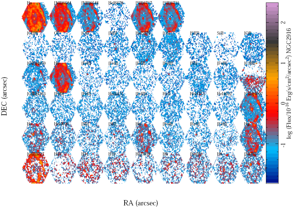
Fig. 14 Flux intensity maps for all the emission lines listed in Table 1 and analyzed following the procedure described in § 3.6, in units of 10-17 erg s-1 cm-2 arcsec-1, derived for NGC 2916. The color figure can be viewed online.
Finally, along this article we have illustrated the average quantities derived from the analysis of the stellar population: luminosity-weighted age and -metallicity, and stellar dust attenuation. However, as indicated in Paper I F 3D provides the full star formation and chemical enrichment histories (e.g., Figure 7 & 9 of that article), and when implemented in P 3D it also provides the corresponding spatially resolved versions of both dataproducts. As an example of this analysis we present in Figure 15 the cumulative stellar mass density (Σ*, t) along cosmological time, i.e., the stellar mass density as a function of lookback time, derived from the stellar population analysis of the CALIFA V500 setup data of NGC 2916. This Σ*, t distribution has been analyzed to determine whether galaxies grow their stellar mass inside-out or out-in, as well as the difference in mass assembly depending on galaxy properties (e.g. Pérez et al. 2013, Ibarra-Mede et al., submitted). We should note here that this procedure is unable to determine where those stars were actually formed. Thus, it is unsensitive to radial movements. However, by describing the spatial distribution of stellar mass at different epochs it shows how the mass is assambled, irrespective of the origin of those stars (in situ star formation or migration).
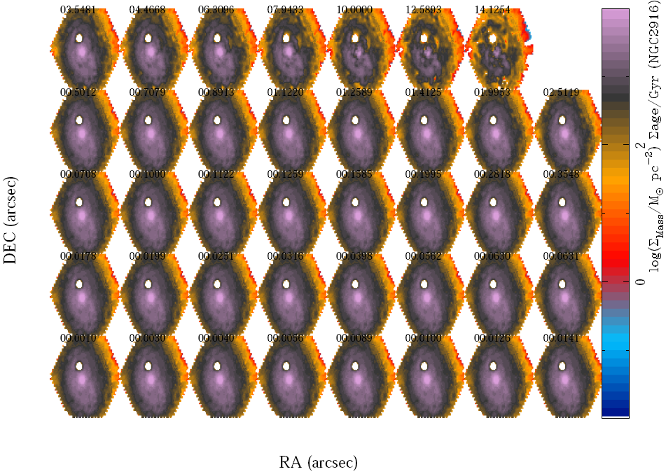
Fig. 15 Cumulative stellar mass density at different lookback times derived from the analysis of the stellar population of NGC 2916. The color figure can be viewed online.
4.1. The properties at the effective radius
Previous studies have reported that some properties of both stellar populations and ionized gas at the effective radius are representative of the average properties of galaxies (e.g. Moustakas et al. 2010; Sánchez et al. 2013; González Delgado et al. 2015). As an example of the practical use of the dataset analyzed here, we will explore this result by comparing five of the main dataproducts de rived by P 3D: The luminosity-weighted stellar log age and metallicity, the dust attenuation of the stellar component, the dust attenuation derived for the ionized gas, and the gas phase oxygen abundance.
The average values have been obtained as the mean values across the optical extension of the galaxies, without a weighing, or rejection process for the stellar population as derived directly from FIT3D (Paper I, § 2.3) and shown in Figure 7. The gas phase dust attenuation was obtained across the optical extension of the galaxy based on the spaxel-by-spaxel Hα to Hβ line ratio and using the prescriptions described in § 4. For the gas phase oxygen abundance we adopted the 03N2 line ratio and the calibrator proposed by Marino et al. (2013). This line ratio involves the use of flux intensities of the following emission lines: [ O ], [ N ], Hα, and Hβ. For both the dust attenuation and the oxygen abundance a 3σ selection criterion was applied to all the emission lines involved in the derivation of the parameters, spaxel-by-spaxel. Once the map of the different properties was derived, the mean value was obtained without any further rejection criteria. Finally, we excluded those average values derived for galaxies that do not have at least 50 spaxels (an area of ≈7 arcsec2) fulfilling the accuracy criteria indicated above to derive the considered parameter. The individual values resulting from this analysis are listed in Appendix B, Table 9.
The values at the effective radius have been derived as the average within an annular ring of 0.75-1.25 effective radius from the center of the galaxy, after deproject-ing the 2D distribution of the parameter. For the effective radius we adopted the value described in Walcher et al. (2014). For the deprojection we adopted the procedure described in Sánchez et al. (2014), using the average semi-minor to semi-major axis ratio and ellipticity calculated from the isophotal analysis described in the Appendix of that article. An intrinsic ellipticity of q o=0.13 has been taken into account in the deprojection procedure. Finally, we excluded those average values at the effective radius derived for galaxies that did not have at least 10 spaxels in the annular ring fulfilling the accuracy criteria indicated above to evaluate the parameter. The individual values obtained by this analysis are listed in Appendix B, Table 10.
Figure 16 shows the comparison between the average values calculated across the optical extension of the galaxies and the values at the effective radius as described before. For each of the parameters we perform a least square linear regression, deriving both the correlation coefficient and the slope of the correlation. In addition, we calculate the reduced X 2/v with respect to the one-to-one relation, and the mean and standard deviation of the difference between the two parameters.
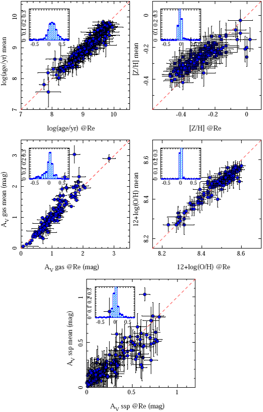
Fig. 16 Comparison of the average value and the value at the effective radius for four properties of the galaxies: Top-left: Luminosity-weighted log age. Top-right: Luminosity-weighted metalliciy. Central-left: Ionized gas dust attenuation. Central-right: gas phase oxygen abundance. Bottom panel: Dust attenuation of the stellar population. For this latter parameter the errors have been truncated to a maximum value of 0.15 mag, for the sake of clarity. In each panel the inset shows the normalized histogram of the difference between the two estimations of the parameter. The color figure can be viewed online.
The results of this analysis are included in Table 7. As expected from the inspection of Figure 16, all the parameters analyzed show a clear and strong correlation, with large correlation coefficients. In almost all the cases the correlation has a slope near to the one-to-one relation, except for the stellar abundance ([Z/H ]), which seems to have a smaller slope. When compared with the one-to-one relation, three parameters (log(age), [Z/H ], and 12+log(O/H)), show a X 2/v near to one, indicating that their correlation is completely compatible with the unity relation. For the gas phase dust attenuation, the X 2/v is too large, taking into account that the two derivations of this parameter present a strong correlation with a slope very close to one. We consider that this is due to a clear underestimation of the error of A v, which requires a re-evaluation, rather than an indication of a clear deviation from the one-to-one relation. Indeed, including a systematic error of 0.15 dex in both parameters, the X 2/v reaches a value near to one. We find the opposite effect for the stellar dust attenuation. It is clear from Figure 16 that the estimated errors are much too large. This may be due to the inclusion of the standard deviation with respect to the mean values in the error budget, which indicates that the individual derivation of the dust attenuation is not very stable at each spatial bin. A global reduction of the estimated errors in these parameters by about ≈50% makes the X 2/v reach a value close to one. In general, the difference between each pair of explored parameters is almost compatible with zero, or shows very small offsets compared with the overall dispersion and the individual estimated errors.
This study demonstrates that at least for the parameters analyzed the values derived at the effective radius are indeed representative of the average values across the entire optical extension of galaxies. In other words, it seems that the effective radius is indeed effective, as already noticed by Sánchez et al. (2013) and González Delgado et al. (2015). This result is particularly important for those IFU surveys that do not cover the entire optical extension for all the sampled galaxies but whose FoV reach at least one effective radius.
5. SUMMARY AND CONCLUSIONS
Along this article we have described the analysis sequence of P 3D, a pipeline based on FIT3D, developed to extract the main properties of the ionized gas and stellar populations from IFS data. In particular we present the different steps and describe the intermediate and final dataproducts for a set of datacubes extracted from the MaNGA and CALIFA surveys. This includes: (i) cube pre-processing; (ii) analysis of the central spectrum; (iii) spatial binning to achieve the required S/N level per spectrum, and a comparison with the most frequently used binning procedure in the field; (iv) detailed analysis of the stellar population based on multi-SSP fitting in each spatial bin, including a description of the derived dataproducts; (v) analysis of the emission lines in the spatially binned spectra; (vi) the required dezonification to recover a spaxel-wise model of the underlying stellar population and a pure emission line datacube; (vii) the spaxel-wise analysis of the strong and weak emission lines, including a comparison between the derived parameters; (viii) the analysis of the stellar indices, showing a comparison/correspondence with the results derived from the multi-SSP fitting procedure; and finally (ix) a description of the format of the derived dataproducts provided by each individual step of the analysis. In summary, we present here the current status of the P 3D pipeline, as implemented to analyze the data from the three major on-going IFU surveys: CALIFA, MaNGA, and SAMI. P 3D produces reliable estimations (as demonstrated in Paper I, § 3) of the parameters analyzed, which are coherent within the differences between the instrumental setups for the three surveys. The use of a single data format for the dataproducts derived will help to make comparisons between the three surveys in a coherent and simple way. P 3D has already demonstrated its scientific validity, since it was used to analyze: (i) the effects of galaxy interaction in the enhancement of the star formation rate and the onset of galactic outflows, employing CALIFA data (Barrera-Ballesteros et al. 2015); (ii) the exploration of the local version of the star forming main sequence in galaxies using CALIFA data (Cano-Diaz et al. in press); and (iii) the exploration of the evidence of the inside-out scenario in the mass assembly history of galaxies, using MaNGA data (Ibarra Mede et al. in preparation).
As a practical implementation we present the dataproducts provided by P 3D for the publicly accessible datacubes of the 200 galaxies that comprise the V500 setup of the CALIFA DR2. We illustrate the content of the dataproducts delivered showing the Hα intensity maps for all of them, as well as the intensity maps of all the emission lines analyzed for NGC 2916, together with the stellar mass assembly history of this galaxy. For all these galaxies we list a set of parameters that characterize their properties, including the integrated stellar mass and star formation within the aperture of the IFU, the mean luminosity-weighted log age and -metallicity, the dust attenuation for the stellar populations, as well as the oxygen abundance and dust attenuation of the ionized gas, both derived across the full optical extension of the galaxies and at the effective radius. Finally, we demonstrate that, as suggested by previous studies, the values at the effective radius are indeed characteristic of the average values of the parameters across the entire optical extension of the galaxies.