1. INTRODUCTION

Current observations of supernovae of type la (SNIa) (^{Riess et al. 1998}; ^{Perlmutter et al. 1999}: ^{Astier et al. 2006}; ^{Riess et al. 2007}; ^{Amanullah et al. 2010}), cosmic microwave background ra diation (CMB) (^{Komatsu et al. 2011}; ^{Larson et al. 2011}; ^{Ade et al. 2014}) and Hubble parameter data (^{Farooq & Ratra 2013}; ^{Sharov & Vorontsova 2014}) indicate an accelerated expansion of the universe; the ɅCDM model is the best model to fit the observational data. The A term corresponds to a cosmological constant (energy density) which is plagued with several fundamental issues (^{Padmanabhan 2003}; ^{Weinberg 1989}), which motivated the search for alternatives models of gravity that could explain the observations.

Massive gravity theories (^{Fierz & Pauli 1939}; ^{Boulware 1972}; ^{Hassan & Rosen 2012a},^b, ²⁰¹¹; ^{Hassan et al. 2012a},^b; ^{de Rham & Gabadadze 2010}; ^{de Rham et al. 2011a},^b, ²⁰¹²; ^{Hinterbichler 2012}; ^{Arkani et al. 2003}; ^{Hinterbichler & Rosen 2012}; ^{Volkov 2012}; ^{Chamseddine & Volkov 2011}; ^{Volkov 2014}; ^{Kobayashi et al. 2014}; ^{Gümrükçüoğlu et al. 2012}; ^{de Felice et al. 2012}; ^{Gümrükçüoğlu et al. 2011}; ^{de Felice et al. 2013a},^b; ^{de Rham et al. 2014}) are old candidates to explain the accelerated expansion of the universe, since the graviton mass could perfectly induce and mimic a cosmological constant term. However, such kinds of theories were considered for long time unsuitable, due to the appeareance of Boulware-Deser (BD) ghosts (^{Boulware 1972}). Recently a nonlinear massive gravity theory was proposed and shown to be BD ghost free (^{Hassan & Rosen 2012a},^b, ²⁰¹¹; ^{Hassan et al. 2012a}), also in the Stuckelberg formulation (^{Hassan et al. 2012b}). A similar theory was also developed (^{de Rham et al}.(^{de Rham & Gabadadze 2010}; ^{de Rham et al. 2011a},^b, ²⁰¹²), sometimes called the dRGT model (after ^{de Rham-Gabadadze-Tolley}, see ^{Hinterbichler. 2012} for a review), again arising cosmological interest in such theories (^{Arkani et al. 2003}; ^{Hinterbichler & Rosen 2012}; ^{Mirbabayi 2012}). Self-accelerating cosmologies with ghost-free massive gravitons were later studied (^{Volkov 2012}; ^{Chamseddine & Volkov 2011}; ^{Volkov 2014}; ^{Kobayashi et al. 2014}; ^{Gümrükçüoğlu et al. 2012}; ^{de Felice et al. 2012}; ^{Gümrükçüoğlu et al. 2011}; ^{de Felice et al. 2013a},^b; ^{de Rham et al. 2014}). Nowadays, there is general agreement that in dRGT models, which are defined with a flat reference metric, isotropic flat and closed FLRW cosmologies do not exist, even at the background level. Nevertheless isotropic open cosmologies exist as classical solutions, but have unstable perturbations. In the case of a non-flat reference metric a ghost free theory exists for all types of background cosmologies (^{Hassan & Rosen 2011}; ^{Hassan et al. 2012a}), though the perturbations are still unstable in isotropic cases (^{Gümrükçüoğlu et al. 2011}; ^{de Felice et al. 2013a},^b).

Although the theoretical aspects of massive gravity have been studied in the last years, the cosmological constraints on observational data have not. ^{Gannouji et al. (2013)} investigated the cosmological behavior in the quasi-dilaton nonlinear massive gravity, and constrained the parameters of the theory with observational data from SNIa, baryon acoustic oscillations (BAO) and CMB.

In order to study some cosmological bounds concerning the free parameters of the theory, we must have a massive gravity theory with a well-established FLRW limit for the reference metric. As shown in ^{Gümrükçüoğlu et al. (2011)} and ^{De Felice et al. (2013a},^b) the perturbations in anisotropic FLRW are stable. Thus, if we suppose that the anisotropies that cure the instability of the model do not greatly affect the cosmic evolution, we can use the results involving isotropic solutions as a first approximation to the stable anisotropic case. For this case the results of ^{Gümrükçüoğlu et al. (2011)} and ^{De Felice et al. (2013a},^b) are a good starting point to study some bounds in the massive gravity theory as compared to recent observational data. In § 2 we present the general massive gravity theory and in § 3 the cosmological equations. In § 4 we present the constraints from H(z) data and in § 5 some bounds on the graviton mass. We state our conclusions in § 6.

2. MASSIVE GRAVITY THEORY

Our starting point for the cosmological analysis is the massive theory for gravity proposed in ^{de Rham & Gabadadze (2010)}, and ^{de Rham et al. (2011a},^b, ²⁰¹²⁾. The nonlinear action includes, besides a functional of the physical metric ɡμv(x), four spurious scalar fields _^ϕa(x) with a = 0,1, 2, 3, called the Stückelberg fields. They are introduced in order to make the action manifestly invariant under diffeomorphism, (see for example ^{Dubovsky 2004}). Let us start by observing that these scalar fields are related to the physical metric and enter into the action as follows:

1

where the fiducial metric fμv is defined, which is written in terms of the Stückelberg fields:

2

Usually ab is called the reference metric and for the purpose of this paper, one can use ab = ηab = (-, +, +, +) when the scheme proposed by dRGT respects Poincare symmetry. Hence the fiducial metric in (1) is nothing but the Minkowski metric in the coordinate system defined by the Stückelberg fields. So we have automatically defined the covariant tensor which Hμv propagates in Minkowski space, and the action is then a functional of the fiducial metric and the physical metric ɡμv.

The covariant action for massive general relativity can be written as:

3

where 𝒰 is a potential without derivatives in the interaction terms between Hμv and ɡμv, which gives mass to the spin-2 mode described by the Einstein-Hilbert term. As observed in ^{de Rham & Gabadadze (2010)}, and ^{de Rham et al. (2011a},^b, ²⁰¹²⁾ a necessary condition for the theory (3) to be free of the Bouware-Deser ghost in the decoupling limit is that -gU (g, H) be a total derivative. The most general covariant mass term which respects this condition is given by³:

4

where αi are constants and the three lagrangians in (4) are written as:

5

6

7

where one has defined the tensor Kvμ= δvμ- ∂μϕa∂vϕbηab In general there are other polynomial terms in K, and the procedure to generate them can be found in ^{Hassan & Rosen (2011)}, ^{Hassan et al. (2012a)}, ^{de Rham & Gabadadze (2010)}, and ^{de Rham et al. (2011a},^b, ²⁰¹²⁾. However, it has been shown that all terms after the quartic order vanish (see also ^{de Rham et al. 2014}; ^{Creminelli et al. 2005}). Notice also that we have maintained the constant term a2 in order to see its consequences on the evolution equations. The case α2 = 0 is pathological, since in this case the linearised theory and the non-linear one have a different number of propagating modes.

3. COSMOLOGY OF MASSIVE GRAVITY

Let us consider an open (K < 0), homogeneous and isotropic FRW universe for the physical metric:

8

where, μ, v = 0,1, 2, 3 and i,j = 1, 2, 3, with X0= t,X1 = X, X2 = Y, X3 = z . Adopting the same ansatz for the Stückelberg fields used in ^{Gümrükçüoğlu et al. (2011)}, ^{De Felice et al. (2013a},^b), i.e:

9

after plugging back (8) and (9) in (3), one obtains the following Lagrangian (^{Gümrükçüoğlu et al. 2011}, ^{de Felice et al. 2013a},^b) for a(t) and f(t), where the overdot denotes the time derivative:

10

where

11

Assuming the matter content (energy-momentum tensor) to be of the form Tvμ = diag [ -ρ_m(t), p _m(t), p_m(t), p_m(t) ] and taking the equations of motion from 𝓛 _g with respect to ƒ we have:

12

where C = f(t) -K /a(t) . The two interesting solutions are given by⁴:

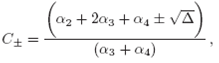
13

where ∆ = α₂ (α₂ + α₃- α₄) + α32 . Moreover, taking the equations of motion from (10) with respect to N and using (13) one obtains the Friedmann equation:

14

where Ʌ± = mg2 ß± , with

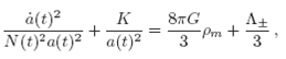
15

a dimensionless parameter depending only on the constants α₂, α₃ and α_4. In (14) one can recognize Ʌ± as the energy density of massive gravity ρ _g. Besides, one expects to obtain the pressure term p _g , in the second Friedmann equation, which can be done by combining (14) with the variation of (10) with respect to a(t), which results in:

16

where H = à(t)/N(t)a(t). Notice that the right hand side of (16) contains only the contribution from the matter part, which indicates that the graviton mass contribution satisfies an equation of state of the form p _g = -p_g, exactly as a vacuum behavior. This same result is also observed in ^{Gümrükçüoğlu et al. (2011)} and ^{De Felice et al. (2013a},^b).

Another combination is possible in order to get a direct relation among ä(t), pressure and energy density (matter and graviton). This time, we eliminate H ² from the equation of motion for a(t). Thus, it is possible to obtain:

17

From (17) it is straightforward to conclude that an accelerated expansion occurs when Ʌ± > 4πG (ρ_m + 3p_m ).

It is also easy to see that Ʌ± acts exactly like an effective cosmological constant in (14). In both Friedmann equations, (14), (16) and also (17), we will set N = 1 in order to reproduce a cosmolog ical scenario. For a positive cosmological constant (which leads to an accelerating universe), we must have Ʌ± > 0, which implies β ± > 0.

From now on we will assume α₂ = 1 according to the original dRGT theory (^{de Rham & Gabadadze 2010}; ^{de Rham et al. 2011a},^b, ²⁰¹²). The Friedmann equation (14) can be rewritten in terms of the present critical energy density ρ _c = 3H02 3/8πG,

18

where H(t) = ȧ/a is the Hubble parameter and Hq ≃ 70 km Mpc/s is its present day value. Writ ing ρ_m = ρ_mo(a/a _o)^-3 , where p _mo is the present day value for the matter energy density, and introducing the density parameters

19

the Friedmann equation (18) can be expressed as

20

or, in terms of the redshift parameter defined by 1 + z = ao/a.

21

where we have used the Friedmann constraint

22

which follows from (18) and (19). Observational data can be used to constrain the values of such parameters and this will be done in the next section.

4. CONSTRAINTS FROM OBSERVATIONAL H(Z) DATA

Observational H(z) data provide one of the most straightforward and model-independent tests of cosmological models, as the H(z) data estimation relies on astrophysical rather than cosmological assumptions. In this work, we use the data compilation of H(z) from Sharov and Vorontsova ^{(Sharov & Vorontsova 2014)}, which is, currently, the most complete compilation, with 34 measurements.

Using these data, we perform a X ²-statistics, generating the xH2 function of free parameters:

23

where Ez≡ HZHo and H(z) is obtained by equation (21).

Since the function to be fitted, H(z) = H _oE(z), is linear in the Hubble constant, H _o, we may analytically project over H _o, yielding XH˜2 :

24

where A ≡ ∑i=1nEi2σ2Hi , B ≡ ∑i=1nEi2Hiσ2Hi ,

C≡∑i=1nHi2σHi2 and Ei ≡ HziHO .

The result of this analysis is shown in Figure 1. As can be seen, the results from H(z) data alone yield nice constraints on the plane Ω _m x Ω _g. The flatness limit, which corresponds to Ω _m + Ω_g = 1, is shown as an straight line on this plane (dashed line in Figure 1). Points on and above this line were not considered, since they correspond to non-open models. One may see that the best fit lies right below this line, indicating that the H(z) data alone favor a slightly open universe.

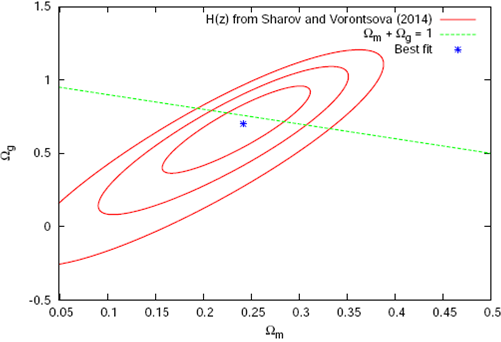
Fig. 1 Solid lines: statistical confidence contours of massive gravity from H(z) data. The regions correspond to 68.3%, 95.4% and 99.7% c.l. Dashed line: flatness limit, where Ω _m + Ω _g = 1. Points above this line are not con sidered in the statistical analysis. Star point: best fit, corresponding to (Ω _m ,Ω _g ) = (0.242,0.703), which leads to Ω _k = 0.055. More details in the text. 

Furthermore, we considered the prior Ωm ≥ Ω _b with the baryon density parameter, Ω _b , estimated by Planck and WMAP: Ω _b = 0.049 (^{Ade et al. 2014}), a value which agrees with big bang nucleosynthesis (BBN), as shown in ^{Olive et al. (2014)}. As a result of this prior, only the 3σ c.l. contour was cut for a low matter density parameter, as we may see in Figure 1.

The minimum X ² was X ² _min = 16.727, yielding a X ² per degree of freedom X ² _v = 0.523. The best fit parameters were Ω _m = 0.242-0.085-0.15-0.19+0.041+0.065+0.090 Ω _g = 0.703-0.34-0.62-0.96+0.069+0.085+0.10 for 68.3%, 95.4% and 99.7% c.l., respectively, in the joint analysis.

As expected, this result agrees with ɅCDM constraints, since this model mimics the concordance model. Moreover, the best fit values of Ω _m and Ωg lead to Ωk = 0.055, which corresponds to a negative value of K, as expected for this model. ^{Sharov & Vorontsova (2014)} found, for ɅCDM: Ω _m = 0.276-0.008+0.009 Ω _Ʌ = 0.769 ± 0.029, Ω _K = -0.040±0.032, for 1σ c.l., by combining H(z) with SN la and BAO data. Given the uncertainties of the massive gravity parameters, the results are in good agreement, even considering the open universe restriction for massive gravity, while ɅCDM has no restriction on curvature.

5. BOUNDS FOR THE GRAVITON MASS

Having obtained the best fit values for the parameters, we show in Figure 2 the plot of massive gravity theory (red line) with a ±1σ limit (red dotted line).

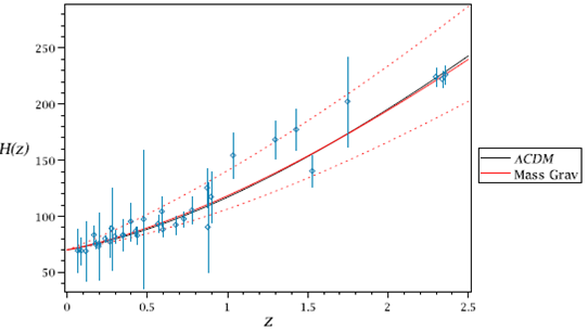
Fig. 2 Plot of H(z) x z for the best fit values of massive gravity theory (red line, from this paper, H(z) data only) with ±1σ (red dotted line). The ɅCDM model is also represented (black line, best fit from ^{Sharov & Vorontsova (2014)}, H(z)+BAO+SNs). The points with error bars are the ^{Sharov and Vorontsova (2014)} observational data. The color figure can be viewed online. 

The ɅCDM according to best fit data of ^{Sharov & Vorontsova (2014)} is also represented (black line).

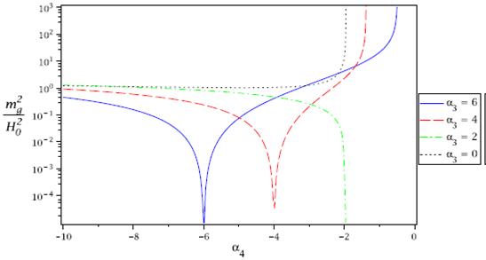
This model also provides an expression for the graviton mass depending on the α ₃ and α ₄ parameters through ß±, namely:

25

If we fix some of the parameters we can see how the mass depends on the others. In Figure 3 we show a typical mass dependence with α ₄ when we set α₃ as a constant and choose to work with β_. Such behavior is also observed for other positive and negative values of α ₃ . It is easy to see that the mass increases and diverges for some specific value of α ₄, corresponding to the limit β_ → 0. In some cases the mass can also abruptly decrease to zero, as shown in the cases α ₃ = 6, α ₃ = 4 and α ₃ = 2. This shows that the graviton mass is strongly dependent on the a parameters, although in the limit of very negative α ₄ values the graviton mass approaches m _g ≃ H _{0 ^-1.}

Fig. 3 Typical mass dependencies on α₄ for some specific values of α₃. 

6. FINAL DISCUSSIONS

In this work we analysed an open FLRW solution of massive gravity which admits an accelerated expansion of the universe, in full accord to observations.

Although massive gravity theories perfectly mimic the ɅCDM model, some important features are very different. The net effect of a finite mass for the graviton is to introduce a constant term proportional to _{^m2 g} in the action (3) (something similar to a potential), which will contribute with a constant term in the motion equations, or Friedmann equations (last terms of (14) and (17)). From a cosmological point of view such a term is very similar to a cosmological constant term, but it also has some important differences. In the ɅCDM model the Ʌ term comes from the zero point energy of the quantum vacuum (although there are important fundamental issues about its magnitude), while in massive gravity theories the corresponding term presents a much richer structure. It is composed of constant terms, α₂, α3 and α ₄ [see (15) ] that are the contributions from the corresponding terms coming from the lagrangians needed to eliminate the Bouware-Deser ghosts present in the theory. From a classical point of view, the α constants are yet unknown. Their values may come from a perturbative quantum construction of the theory. A theoretical approach in order to obtain the values of such constants would certainly represent a great advance in the field.

The constraints from recent observational H(z) data were found, and the best fit values obtained for the cosmological parameters were (Ω_m, Ω_g, Ω_K ) = (0.242, 0.703, 0.055). The values obtained for Ω _m and Ω _g at 1σ were in good accord to the best fit values found by ^{Sharov & Vorontsova (2014)} for the ɅCDM model (see the end of § 4), although the ɅCDM model points to a slightly closed universe (Ω_k = -0.040) and our best fit indicates an open universe (Ω _k = 0.055). This is an important difference between the models, but it is also important to note that the massive gravity theory is valid only for an open universe (^{Gümrükçüoğlu et al. 2011}, ^{de Felice et al. 2013a},^b), while ɅCDM has no restriction on curvature. As ɅCDM and massive gravity theories have the same background behavior, at least for an open universe, we do not expect to find differences between both models if we use as constraints the CMB shift parameter or the BAO scale. However, a full density perturbation analysis of the massive gravity model could lead to differences with respect to ɅCDM, which could be evidenced by the full CMB spectrum or by the matter power spectrum. This analysis will be presented in the future.

It is also important to analise the graviton mass dependence on the parameters α ₃ and α ₄ of the model (α₂ can be normalized to 1). We verified that a strong dependence on such parameters is evident. The mass of the graviton is present in Ω _g [ see (19) ]. and we can see that the observational constraints are not enough to furnish the graviton mass. According to (25), just by setting specific values for the α's (or for β) we can estimate the graviton mass with the best fit of Ωg. In view of such restrictions, even considering other observational data such as BAO or CMB, we will only obtain best fit values for Ω _g, with no new information about the graviton mass.

An interesting relation between the graviton mass and the α parameters is shown in Figure 3. For some integer values of α ₃ and α ₄, the β parameter approaches infinity (specifically α ₃ = -α₄), and for others it approaches zero, allowing very small and very huge values for the graviton mass near such points. Only by theoretically obtaining such parameters could the graviton mass be better estimated. We have also verified that for several values of positive α₃ and negative α ₄, the ratio m _g/Ho≃ 1, indicating that for such values the graviton mass is m _g ≃ H ₀ ^-1 ~10 ^-33eV. Such a value is much closer to the mass of quintessence models, where a scalar field is introduced by hand in order to interpret the dark energy as a scalar field fluid. To attribute a mass to the graviton is certainly a more appealing theory than the introduction of new kinds of fields.