text new page (beta)
 English (pdf)
 Article in xml format
 Article references
 Send this article by e-mail
 Cited by SciELO
  Similars in
SciELO
Similars in
SciELO 
 Permalink
1. INTRODUCTION
V1309 Sco underwent a nova-like outburst in 2008 (Nakano 2008). Its characteristics were similar to those of the eruptions in V838 Mon in 2002 (Munari et al. 2002), V4332 Sgr in 1994 (Martini et al. 1999) and several extragalactic objects (Mould et al. 1990; Kulkarni et al. 2007; Berger et al. 2009). Soker & Tylenda (2003) proposed that the energy source of these events could be the merger of two low-mass stars, an idea that is now strongly supported by the events leading up to the V1309 Sco eruption and its subsequent observations.
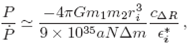
The pre-outburst state of V1309 Sco was observed fortuitously by the OGLE-III and OGLE-IV3 projects starting in 2001. These data, analized by Tylenda et al. (2011), indicate the presence of an eclipsing binary whose orbital period rapidly decayed: during 2002-2004, P/Ṗ
The orbital evolution immediately prior to the merger was modeled under the assumption of angular momentum loss through magnetized stellar winds during two-thirds of the system's lifetime, followed by Roche lobe overflow (Stepieh 2011). This model implies that during the time of the OGLE observations, V1309 Sco was already a contact system with the stars filling their Roche lobes.
In this paper we explore an alternative scenario that does not require mass loss nor that the stars be already filling the Roche lobe during the early phase of the period decline. Instead, we make use of the fact that, as a star expands during post-main sequence evolutionary phases, the rotation rate of its outer region becomes sub-synchronous, leading to tidal shear energy dissipation. We thus explore the possibility that the observed orbital decay in V1309 Sco was a consequence of this mechanism. We find that the behavior of P/Ṗ over the timescale during which this quantity was measured can indeed be reproduced in a straightforward manner with the tidal shear energy dissipation scenario. The method and assumptions are described in § 2. The results are presented in § 3 and discussed in § 4.
2. TIDAL SHEAR ENERGY DISSIPATION
The only basic facts known about V1309 Sco prior to its outburst are: (a) Teƒƒ =4500 K, suggesting the presence of a solar-type star in the system: (b) a periodic light curve with two eclipses during the observations of 2002-2006 and only one eclipse at the end of the 2007 observing season; (c) a distorted light curve indicating a tidally deformed stellar shape; and (d) a systematically decreasing trend in the period, with P/Ṗ ≃1000 years during 2002-2004 and 170 years during 2006-2007.
Taken together, these facts indicate that we witnessed the end stages of physical processes that initiated slowly and accelerated over time. Consider the process by which a binary star evolves when it leaves the main sequence (MS): In general, as the core contracts, the outer region expands and assuming conservation of specific angular momentum, the rotation angular velocity of these layers decreases. Hence, a star that had attained synchronous rotation during its MS lifetime now becomes sub-synchronous (in its outer region). If the rate of expansion is faster than the synchronization timescales, then the star remains sub-synchronous for the remainder of the expansion phase.
As soon as the star becomes sub-synchronous, tidal shear energy dissipation becomes active. The amplitude of tidal perturbations and the energy dissipation rate increase rapidly with increasing stellar radius and/or decreasing orbital separation. In an equilibrium state, the energy that is deposited in the stellar layers as heat is transported outward and eventually lost through radiation. However, if the rate of shear energy dissipation is too large, the star becomes bloated, an outcome that has been analyzed for a variety of objects, including white dwarfs (Dall'Osso & Rossi, 2014) and planets (Bodenheimer et al. 2001; Gu et al. 2004; Leconte et al. 2009).
The bloating contributes to keep the rotation sub-synchronous and the tidal forces not only remain active but become more intense with each radius increase. Hence, the outcome of this process is most likely a runaway phenomenon. This is the scenario that we explore for V1309 Sco in the following sections.
2.1. Model and assumptions
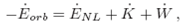
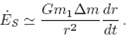
The simplest model to assume is one in which V1309 Sco consists of a 1 Mʘ primary star (m 1) that has recently left the main sequence. The companion is chosen4 to be of 0.8 Mʘ. As described above, the expansion of the primary's outer region has caused its rotation rate to become subsynchronous with respect to the orbital period, leading to tidal shear energy dissipation, Ės. This quantity, when added to the the rate of change of the rotation energy, Ḱ, and of the gravitational potential energy, Ẇ, must be compensated by a the change in orbital energy:
 1
1
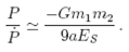
Using the expression for the orbital energy E orb = -Gm 1 m 2/2a and assuming no mass loss we have:
 2
2
where a is the orbital major semi-axis and G the gravitational constant. With Kepler's relation, a 3 = (G/4π2)(m1 + m2)P2, we can then write
 3
3
Assuming that the three terms of the right of equation (1) are approximately equal to each other leads to Ės ≃ - Eorb/3, and
 4
4
and thus.
 5
5
We compute Ės in the surface layers of m 1 as they respond to the presence of m 2 using the TIDES code (Moreno & Koenigsberger 1999; Moreno et al. 2011). The assumption is made that the lower-mass companion m 2 has not yet reached the end of its main sequence lifetime and thus it remains synchronous throughout the process that we describe.
The TIDES code computes Ė s by solving the equations of motion for a grid of volume elements that constitute a shell S at radius r which encloses the mass m 1. The main body of m 1 interior to S is assumed to behave as a rigid body and the tidal deformation is assumed to occur only in S. The equations of motion include the gravitational forces of m 1 and m 2, and Coriolis, centrifugal, gas pressure and viscosity forces on m 1. The stellar equator is assumed to lie in the orbital plane and m 2 is treated as a point source.
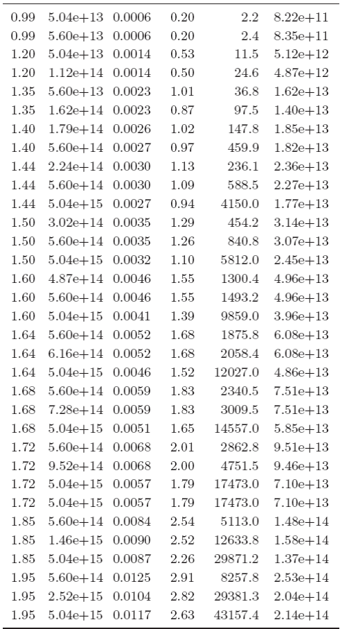
Values of Ės are obtained for a set of successively increasing stellar radii, as listed in Column 1 of Table 1 which, when substituted into equation (5) provide values of P/Ṗ. Each radius is assumed to correspond to a different point in time. In this manner, the expansion of the star is taken into consideration. However, the actual rate of expansion is a priori not known. In order to estimate it, we use the rate of change of the gravitational potential energy Ẇ, due to the expansion of the shell S whose mass is ∆m, and, assuming no mass loss.
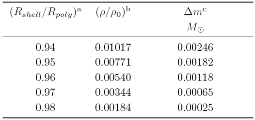
Table 1 Results: nominal case
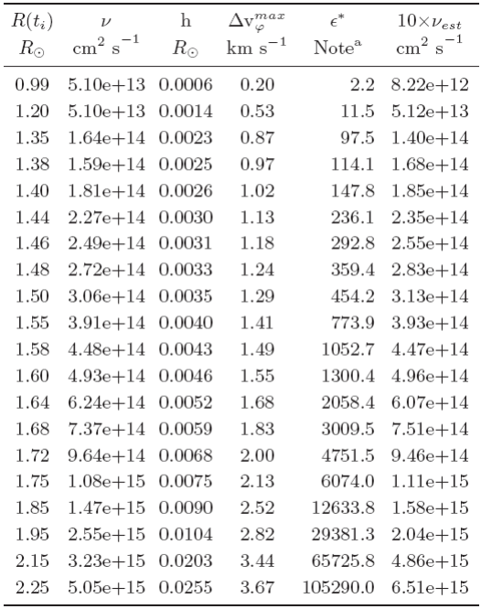
aϵ* is in units of 1035 p ergs/(s - g/cm3 ), where p is the mass density.
 6
6
where m r is the mass interior to the radius r of S. Making use of the approximation Ẇ ≃ Ė s and taking mr ≃ m 1, since the mass contained in S is negligible compared to the total mass below it, we can write
 7
7
Thus.
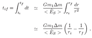 8
8
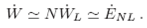
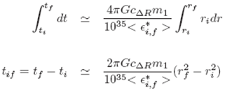
which gives the time it takes the shell S to expand from ri to r f, due to the energy input < Ė s >, the latter being the average of the computed Ė s values at ri and r f. The time that has elapsed since an initial epoch to is then
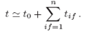 9
9
2.2. Input parameters
The input parameters for the Ė s calculation are the stellar masses (m 1,m 2), the radius r i of S, the synchronicity parameter (β 0 =ω/Ω0), the orbital period and eccentricity (P,e), the kinematical vis cosity (v), the equation of state, the thickness of S (c∆ R ri), the grid size (N φ, Nθ), the tolerance for the Runge-Kutta integration of the equations of motion (Tol), and the number of orbital cycles needed to reach the stationary state (N cycle ).
For V1309 Sco, we adopt m 1 = 1Mʘ, m 2=O.8Mʘ, P=1.44d, e=0, β 0 = 0.95, c∆ R = 0.02. The equation of state is assumed to be polytropic, p = po(ρ/ ρo) γ' , with γ' = 1+ 1 = /n,n the polytropic index and ρ the mass density. For the present calculations we used n = 1.5, following the suggestion of Press et al. (1975) who note that the temperature gradient in asynchronous binaries ought to be nearly adiabatic rather than that given by radiative opacities, so that the turbulent envelope should be roughtly an n = 3/2 polytrope.
All computations are performed with a grid size (N φ, Nθ)=(500,20) which covers half a hemisphere from the equator to a co-latitude of 85°. The tolerance of the Runge-Kutta integration scheme was chosen Tol=10-11-10-7, depending on the particular case, and N cycle =37.
The largest uncertainty in the input parameters involves the choice of v, the kinematical viscosity. The standard molecular viscosity is ≃1-105 cm2s-1. orders of magnitude smaller than the values typically used in models of astrophysical phenomena (Adame et al. 2011; Alexander 1973; Sutantyo 1974; Hansen 2010; Penev et al. 2007) or derived from observational data (Pérez de Tejada 1999). The general idea is that turbulence can enhance by many orders of magnitude the value of v. Although progress is being made in understanding the turbulent viscosity (c.f., Penev et al. 2007; 2009 for stars; Ogilvie & Lesur 2012 for protoplanetary disks), the actual value for the viscosity to be used in particular problems is still unconstrained.
A standard expression for the turbulent viscosity involves the definition of a length scale, h, associated with the size of the turbulent eddies, and a velocity scale, v turb, which is the typical velocity of these eddies. For accretion disks, a simple parametrization of these two scales was proposed by Shakura & Sunyaev (1973). For the length scale, they assumed isotropy and characterized it by the typical size of the largest turbulent eddies, which cannot exceed the local pressure scale height, H. For the velocity scale they reasoned that if the turbulent velocity were su personic, the associated shock waves would have the effect of dissipating energy and thus reducing the velocity to the sound speed, c s, or smaller. Hence, v turb ≤ cs. From these considerations, they arrived at the α-prescription for the viscosity: v ≃ αHc s, where α takes on values 0-1.
Guided by these ideas, we explored the use of the following prescription for estimating v.
 10
10
where h is the height of the major bulge in the equilibrium tide approximation and ∆vφ max is the maximum azimuthal velocity perturbation. α T is a parameter that takes into account factors that are additional to the tidal perturbation, such as magnetic fields and convection, as well as the timescale for the propagation of perturbations. Considering that the latter is the sound speed, c s, an analogy with the Shakura & Sunyaev (1973) prescription provides a rough estimate α T ∆ vφ max ≃ c s. Since ∆ vφ max << c s, we expect α T >> 1·
2.3. Method of computation
A set of stars with radii r i in the range 0.99 - 2.25 R ʘ was chosen for computation with TIDES, using a shell thickness c∆ R ri =0.02r i .
The computations were conducted in two steps. In the first step, v was chosen close to the smallest value that allows TIDES to arrive at a stationary solution. 5 This computation provided a first set of values of h and ∆ vφ max . Considering that cs ≃ 20 - 30 km s -1 (Guenther et al. 1992; for a shell located at 0.98Rʘ in a standard solar model) and that ∆ vφ max ≃ 2 - 3 km s-1 (see below), we adopted α T =10 for ri >1 R ʘ. This yielded the values of v (Column 2 of Table 1) that were used in the second step.
The values of h and ∆ vφ max obtained in the second step calculation are listed in Columns 3 and 4 of Table 1, and Column 6 lists the corresponding values of v est. The differences between these new values and the ones obtained in the previous step are minor. This is because h and ∆ vφ max do not depend strongly on the chosen value of viscosity.
The output of the TIDES calculation is the quantity
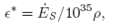 11
11
where Ės/1035 is the energy dissipation rate in units of 1035 ergs s-1 and p is the average mass density in shell S in units of g cm-3. The values of ϵ* that were obtained are listed in Column 5 of Table 1.
Equations (6) and (9) require ∆m, the mass contained in S, and its average density, p, for which a stellar structure model is required. As will be seen below, the timescale over which tidal shear energy dissipation can cause a layer to expand is very short compared to evolutionary timescales. Stellar evolution models for low-mass stars do not contemplate such short timescales because changes in a single star occur over much longer times. For example, it takes the radius of a post-main sequence 1 Mʘ star 16.6 Myr to increase from 2.50 to 2.55 Rʘ. Furthermore, it is not even clear whether a stellar structure model for a single star is a valid approximation for a tidally perturbed star. Hence, in what follows, we first adopt the hypothesis that the outer layers of an asynchronous binary star can be approximated with a n=1.5 polytropic structure (Press et al. 1975), which provides p and ∆m. In the second approach, no assumption is made concerning the manner in which the outer layers expand, thus allowing for an arbitrary density structure. Ė s is obtained by adjusting the parameter N∆m, which is the total mass involved in the energy dissipation and expansion processes.
2.4. Polytropic structure
The stellar structure of 1 Mʘ n=1.5 polytrope was computed for stars of radii Rpoly =1-2.3 Rʘ. These models provide ρo, the central density and (ρ/ρ0) shell, the relative density, as a function of shell radius, R shell. The nature of polytropes is such that, given a stellar mass, ρ/ρo is constant for a fixed value of R shell /Rpoly, for all R poly. Furthermore, ρ 0 = p1(Rpoly1/ Rpoly )3 , where ρ 1 is a reference central density, here chosen to be that of the R poly1 = 1 R ʘ model, ρ 1 =8.453 g/cm3. Hence, for each shell radius, the density is
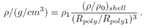 12
12
We list in Table 2 the value of (ρ/ρo) shell for the base of shells located at R shell /Rpoly=0. 94, 0.96, 0.97, 0.975 and 0.98. Also listed in this table is ∆m, which is constant for a shell located at a fixed R shell /Rpoly, of thickness c ∆R Rpoly for all R poly, with a constant c∆r.
2.5. Arbitrary density variation in expanding layers
It is possible to circumvent the use of ρ and ∆m required by equations (5) and (9) by defining a layer L that is larger than the shell S that we model, and by assuming that the mass contained within L remains constant as the star (and the layer) expands. We assume that there is a number of such layers, N. and that the mass involved in both the tidal shear energy dissipation process and in the expansion process is N∆m. In the Appendix we provide the details of the mathematical manipulations that allow us to write P/Ṗ in terms of N∆m and which yield t which is independent of the unknown ρ and ∆m values.
3. RESULTS
3.1. Polytropic structure
We explored the behavior of polytropic shells at various depths by comparing the trend of P/Ṗ vs. t from equations (5) and (9) with that which is derived from a fit to the observations. Specifically, Tylenda et al. (2011) find that the observed variations of P over the time span 2002 to 2007 are given by P/d = 1.4456 exp [ 15.29/(t -t0) ], with t 0 = JD = 2455233.5 and t < t 0. Thus,
 13
13
The uncertainty δ(P/Ṗ) in this relation can be derived by propagating the uncertainties given for P and t on Tylenda et al.'s Figure 2. We find that at JD = 24452870 and JD = 24454250, δ(P/Ṗ) ≃51 and 5 yr, respectively. The uncertainty δt ≃50 and ≃10 d is the same as given in this figure. The above-stated times correspond to P/Ṗ=1000 and 170 yr, respectively. The curve from equation (13) and the associated uncertainty (dashed line) are plotted in Figure 1 and compared to the results derived from the tidal energy dissipation calculations.
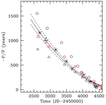
Fig. 1 Trend of P/Ṗ over time t for 1 M ʘ poly tropic stars of radii R poly, for shells located at 0.94R R poly (triangles), 0.95R poiy (squares) and 0.96R R poly (pentagons). Also shown is the result for the approximation described in the Appendix, with N∆m=0.0016 M ʘ (stars). The solid curve corresponds to the observational constraints (equation 13). The error bars located at JD = 24452870 and JD = 24454250 correspond to the propagated uncertainty from the error bars in Figure 2 of Tylenda et al. (2011). The dashed curves are indicative of the uncertainty over the range of dates shown in the figure. Model data were shifted along the time axis so as to coincide with the curve around JD = 2454250, where the propagated uncertainties on the observations are smallest.
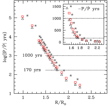
Fig. 2 P/Ṗ for 1 M ʘ polytropic stars for shells located at 0.94R poly (triangles) and 0.95R poly (squares). Also shown is the NAm approximation (stars) described in the Appendix. The dotted lines enclose the region cor-reponding to the observations reported in Tylenda et al. (2011), providing the range in R poly values that corre spond to the dates of observation. The inset shows the same data on a linear scale for P/P <1600 yr.
The best agreement is obtained with a polytropic shell whose base lies at 0.95 R poly. Shells that are deeper or more superficial diverge significantly from the observational curve. As listed in Table 1, this shell contains ∆m=0.0018 M ʘ. During the timeframe in which the orbital period was observed to decay, our results indicate that the stellar radius increased from ≃1.6 R ʘ to 1.8 R ʘ, as illustrated in Figure 2.
Table 3 lists the values of the physical quantites that were computed using the polytropic stellar structure approximation for R shell/Rpoly=0.95. Columns 1 and 2 contain, respectively, the radii at t i and t ƒ ; Columns 3 and 4 contain Ės for the respective radii; Columns 5 and 6 contain the corresponding P/Ṗ; Column 7 lists the time required for the shell to expand from R(t i ) to R(t ƒ ); and Column 8 lists t, the time that has elapsed since the star first became asynchronous. We will refer to this case as the nominal case.
3.2. Arbitrary density variation in expanding layers
Equations (18), (22) and (9) were used with the data of Table 1 to obtain the trend in P/Ṗ vs. t for a broad range in N∆m values. The best match to the observations was attained with N∆m=0.0016 M ʘ. a value remarkably similar to that obtained in the nominal case described above. These results are also plotted in Figure 1 and listed in Table 4. During the epoch for which observations are reported, the stellar radius is found to have increased from ≃1.60 R ʘ to 1.85 R ʘ, which is also consistent with the result of the nominal case.

3.3. Dependence on m 2 , v and polytropic index
Additional calculations were performed to explore the dependence on m 2, v and polytropic index, n. Each of these input parameters was changed, one by one, keeping the others fixed.
The results obtained from the grid of calculations for n = 3 yielded values of ϵ* that differed from those of the nominal case by <4 % for R <2Rʘ. For the cases run with R >2R ʘ the differences increased up to 13%, with the n = 3 cases resulting in larger values of ϵ* ; this, however does not significantly modify the results obtained with the nominal case.
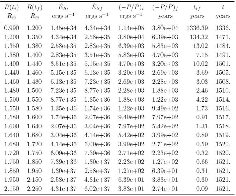
The results obtained from a grid of calculations with m 2=0.4 Mʘ show that the energy dissipation rate decreases by a factor of ≃2 for R <2 Rʘ, i.e., proportional to the decrease of m 2. As a conse quence, for a given radius of m 1, the azimuthal velocity perturbations and the energy dissipation rates are significantly smaller than those of the nominal case, as shown in Figure 3.
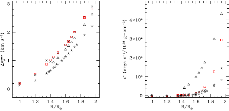
Fig. 3 Dependence of the azimuthal velocity, ∆vφ (left) and energy dissipation rate per unit density (right), as a function of radius and value of m 2 and v. Square: 10 xvest, as in Figures 1 and 2; Cross: v min, approximately the smallest value for which the code runs for that particular radius; Triangle: v ≃9x v min ; Star: m 2=0.4 M ʘ.
Computations were performed using a range of v values, starting with the smallest value that allows the code to run. The results of these computations are listed in Table 5 and show that for R <1.7 Rʘ, ϵ* is directly proportional to the value of v. For larger radii an increase in v leads to a smaller increase in the value of ϵ*. This is because very large viscosities reduce the amplitude of horizontal motions which, in turn, lead to smaller energy dissipation rates.
Table 5 Viscosity dependence
* Results obtained from computations using different values of v while holding all other input parameters constant.
aϵ* is in units of 1035 ρergs/(s - g/cm3), where ρ is the mass density.
Using the approximate linear proportionality for R <1.7 Rʘ, we scaled the ϵ* obtained in the nominal calculation by factors of 0.1 and 5, to obtain approximate results for viscosities v=v est and v= 50vest, respectively.6 The derived trend in P/Ṗ vs. t in the polytropic approximation is plotted in Figure 4, which shows that the viscosity used in the nominal case does indeed provide the best coincidence with the observations.
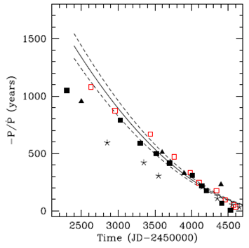
Fig. 4 Comparison of results from runs with values of v and m 2 different from the nominal case (open squares). The curves are the same as shown in Figure 2. The other symbols correspond to: v = 50v est (filled rectangles), v = v est (triangles), and m 2 = 0.4 M ʘ (stars).
The results of these tests are summarized in Table 6. Case 1 is the nominal case, which comes closest to reproducing the observations, and yields P/Ṗ values that go from -1000 yr to -170 yr over a ≃5 year timescale. Case 3 has a viscosity larger by a factor of 5 and the timeframe for the period decay for R >1.40 is consistent with the observations, but there is a significant discrepancy for smaller radii.
Table 6 Dependence on v and M 2
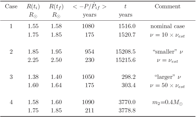
Cases: 1 is the nominal case (i.e., computed with v = 10v est); Cases 2 and 3 are obtained by assuming that Ės is directly proportional to v and using data from Table 1; Case 4 is computed with the nominal input parameters except for m 2 = 0.4Mʘ.
Case 2 has a viscosity smaller by a factor of 10 with respect to the nominal case, and the time required for P/Ṗ to cover the observed range is > 7 yr, significantly longer than in the other two cases. Case 4, which was run with m 2=0.4 Mʘ and the viscosity of the nominal case also has significantly longer timescales than observed. This does not, however, eliminate the possibility of a smaller m,2, but a grid of models for m,2 ≃0.4 (and other values) needs to be constructed using a range of values of v in order to estimate constraints for the secondary mass.
4. DISCUSSION
We propose that the orbital period decline observed in V1309 Sco was powered by tidal shear energy dissipation, Ė s. This mechanism first becomes active when the radius of the initially synchronously rotating star increases as it leaves the main sequence causing outer stellar layers to become subsynchronous. Initially, Ė s is very small and P/Ṗ is very large, but as the radius increases, the rate of period decline accelerates. The heat deposited in the stellar layers due to Ė s contributes to the rate of increase of the radius, thus eventually producing a runaway process where each radius increase results in an increase in Ė s which, in turn, powers an additional radius increase.
V1309 Sco is assumed to consist of a 1+0.8 Mʘ binary, the more massive component having left the main sequence and having a subsynchronous rotation rate. Our calculations of Ė s produce the same trend in P/Ṗ as that observed over the 2002-2007 timeframe and indicate that the radius increased from ≃1.55 to 1.8 R ʘ during the 5 years in which eclipses were evident. The subsequent evolution would have involved an ever more rapid radius increase until Roche lobe dimensions were attained. Note that such rapid radius growth is impossible from evolutionary considerations. For example, grids given by Marques et al. (2008)7 show that the time it takes the radius of a 1 Mʘ star in its latest post-main sequence phases to increase from 2.50 to 2.55 R ʘ is 16.6 Myr.
It is interesting to note that, within the assumptions of the processes and the approximations in the calculation, the mass involved in producing the observed P/Ṗ rate is only ≃0.0016 Mʘ, i.e., approximately 10% of the mass in the outer convective region. One may speculate that this amount of mass should increase as the orbital separation shrinks beyond that which we have computed, thus accelerating the process by which the Roche lobe dimensions are attained.
The method we employ for the computation of the tidal shear energy dissipation, Ė s, is limited primarily by the fact that it neglects the presence of shells above the one being modeled, and that it neglects the perturbations of the layers below it. The absence of a shearing layer above implies that Ė s is underestimated, particularly since the amplitude of perturbations increases with increasing stellar radius. This, however, may be partly compensated by the overestimate of Ės produced by the assumption of a rigidly rotating region below.8 A multilayer calculation would extend the energy dissipation and heating of the stellar material to deeper regions of the star and thus involve a larger fraction of the convective zone in the dissipation/expansion process. The ideal solution is a full 3D computation of the tidal perturbations combined with the evolution of orbital parameters and stellar rotation, which however, is currently not tractable.
It is also interesting to note that the timescale from the start of subsynchronous rotation to the phase of runaway radius increase leading up to the Roche lobe overflow dimensions is extremely short, a few thousand years. This suggests that objects such as V1309 Sco might be relatively common, as recently concluded by Kochenek et al. (2014), although the probability of observing them during this phase is likely to be very small due to its short duration. Clearly, the actual rates will depend on the distribution of orbital separation, on the component masses and, not least, on the opacity and viscosity of the surface layers. For example, we estimate that if v is a factor of 10 smaller than that used in the nominal case, the timescale between the start of asynchronous rotation and the observed orbital period decay becomes a factor of ≃10 larger.
We find a convenient scaling for the viscosity v = αt h ∆v φ max, where h is the height of the major bulge in the equilibrium tide approximation, ∆v φ max is the maximum azimuthal speed of the tidal flow and αt is a parameter that takes into account factors other than the tidal perturbations, such as magnetic fields and convection. Accordingly, since h and ∆v φ max depend on the stellar and orbital parameters, the value of v also depends on these quantities, an idea first suggested by Press et al. (1975). To achieve the agreement between our calculations and the observational constraint shown in Figure 1, we used αt =10, resulting in v = v(r) = 1013 - 1015 cm2/s, with the larger values corresponding to larger radii.
The nature of tidal perturbations is such that their amplitude is largest in the equatorial plane, declining towards the polar ragions.9 Hence, an interesting problem concerns the manner in which the energy that is deposited near the equatorial region due to tidal shear may affect the stellar structure. Relevant to the V1309 Sco event is the question of whether the increasing tidal shear energy dissipation rates have an impact on mass loss. Dynamical models (e.g., D'Souza et al. 2006) predict significant mass-loss associated with a merger. However, there might have been circumstellar matter present in the V1309 Sco system well before the outburst (McCollum et al. 2014). One may speculate that, in addition to triggering the initial orbital period decay the tidal instabilities may provide sufficient energy for mass loss along the equatorial plane, well before the merger occurs.