


 nova página do texto(beta)
 Inglês (pdf)
 Artigo em XML
 Referências do artigo
 Enviar este artigo por email
 Citado por SciELO
  Similares em
SciELO
Similares em
SciELO 
 Permalink
1. INTRODUCTION
Measurements of the Hubble constant H o are crucial for the establishment of a cosmic concordance model in cosmology. This constant plays a role in most of cosmic calculations, such as those about the age of the Universe, its size and energy density, primordial nucleosynthesis, the physical distances between objects, etc. Its importance will even increase in the next decade, since new missions and observational projects are currently being designed to provide accurate measurements of the Hubble constant, e.g., improved parallax calibration for Galactic Cepheids with Spitzer and GAIA, and 1% precision of H o with LISA based on the gravitational radiation from inspiraling massive black holes, which would also increase the precision of the other cosmological parameters.
There are several ways to determine H o by using low and high-redshift sources. The most common methods are based on the period-luminosity relation of cepheids, the tip of the red giant branch (TRGB) and the type la supernovae (SNe Ia) observed in the local Universe (Freedman & Madore 2010). However, some alternative procedures, such as the Sunyaev-Zel'dovich effect combined with X-ray emission from clusters, which allow a measurement of H o from high-redshift objects, have also been discussed (Cunha et al. 2007; Holanda et al. 2012).
Actually, independent estimates are needed in order to obtain a reliable value for H o that is not plagued by systematic errors arising from astrophysical environments, as well as from calibrations related to the cosmic distance ladder. In this regard, the importance and cosmological interest of different estimates of H o that are independent of the distance ladder has also been discussed by many authors (see Jackson 2007, and references therein for a recent review).
Recently, a tension was reported between the value obtained by (Riess et al. 2011) of H o = 73.8 ± 2.4 km s-1 Mpc-1 (1σ), based on measurements of cepheids and SNe la (or al ternatively, that of Freedman et al. 2012, who obtained H o = 74.3 ± 2.1 km s-1 Mpc-1 (1σ), and the value released by Planck of H o = 67.3 ± 1.2 km s-1 Mpc־1 (1σ), Ade et al. 2014), obtained from measurements of the anisotropies of the cosmic microwave background (CMB). The former is based on local measurements, while the latter assumes a cosmological model to infer H o. There are several possible explanations of this discrepancy, such as the following: we live in a Hubble bubble and the local value of H o is subject to cosmic variance (Marra et al. 2013); or there is a problem in the calibration of the cepheids and the true value of H o is lower, as given by (Sandage et al. 2006); or with the TRGB and SNe la given by (Tammann & Reindl 2013); or an extension beyond the standard model of cosmology is needed.
In fact, it is the last option which must be considered, since the emergence of the ɅCDM model as the concordance model in 1998, based on the SNe la observations (Riess et al. 1998; Perlmutter et al. 1999), brought with it the cosmological constant and the coincidence problems. As a complete and convincing solution to these problems is still unknown, it is very important to test all the hypotheses of the model. In addition, it is important to verify that different analyses give the same results, since several kinds of data covering different cosmic epochs are available.
In this regard, a possible alternative procedure to measure H o is to consider the Lyman-α (Lyα ) forest data and the acoustic peak caused by the baryons acoustic oscillations. The Lyα forest probes the low density intergalactic medium (IGM) over a unique range of redshifts and environments, as seen in the spectra of high-redshift quasars. The observed mean transmitted flux depends on the local optical depth, which in turn depends on the expansion rate of the Universe H(z) and some properties characterizing the intervening medium along our line of sight to any quasar. In principle, the values of some cosmological parameters, including the Hubble constant, could be constrained if we had a moderate knowledge of the IGM properties, such as the hydrogen photoionization rate and the mean temperature, and combined this information with the BAO measurement.
In the last decade, several studies have been performed using Lyα forests as cosmological tools (Mc-Donald et al. 2000; Weinberg et al. 2003; Wyithe et al. 2008; Viel et al. 2009). Some works use the flux power spectrum of the Lyα forest to infer the cosmological parameters in two ways: inverting the flux power spectrum to estimate the underlying dark matter power spectrum (Croft et al. 1998, 1999; Hui 1999; Nusser & Haehnelt 1999), or using the power spectrum directly (McDonald et al. 2000; Mandelbaum et al. 2003; McDonald et al. 2005). More recently, new possibilities for using Lyα forests for cosmological purposes were created by the detection of baryon acoustic oscillations in the correlation function of the transmitted flux fraction (Busca et al. 2013; Slosar et al. 2013).
A simpler approach is to use a semi-analytical model to describe the IGM as proposed by (Miralda-Escudé et al. 2000), who derived a fitting formula for the distribution function of volume density in agreement with simulations that yielded similar results for different numerical methods and different cosmologies (Rauch et al. 1997). This allowed to estimate a theoretical mean transmitted flux and to compare it with observational data in order to constrain the cosmological parameters.
Assuming a flat ɅCDM cosmology, we applied the above described procedure for deriving crosscheck values for the Hubble constant H o and the matter density parameter Ω m. Based on two independent samples of Lyα forest data compiled by (Bergeron et al. 2004) and (Guimarães et al. 2007), respectively, we performed two distinct statistical analyses. First, we considered only the Lyα forest data set, while the second approach involved a joint analysis combining the Lyα forest data with the measurements of the baryon acoustic peak from the WiggleZ survey (Blake et al. 2012). As we shall see. the degeneracy in the free parameters defining the (h, Ω m) plane is naturally broken when the Lyα data are combined with standard ruler datasets as given by the baryon acoustic oscillations, thereby providing a new independent method to estimate the Hubble constant.
2. THE FOREST SAMPLES
As remarked earlier, in the present analysis we considered two different samples. The first sample consisted of 18 high-resolution high signal-to-noise ratio (S/N) spectra (2.2 ≤ z em ≤ 3.3). The spec tra were obtained with the ultraviolet and Visible Echelle Spectrograph (UVES) mounted on the ESO KUEYEN 8.2 m telescope at the Paranal observatory for the ESO-VLT Large Programme (LP) 'Cos-mological evolution of the Inter Galactic Medium' (Bergeron et al. 2004). The spectra were taken from the European Southern Observatory archive and are publicly available. This program was devised for gathering a homogeneous sample of echelle spectra of 18 QSOs, with uniform spectral coverage, resolution and signal-to-noise ratio suitable for studying the Lyα forest in the redshift range 1.8 - 3.1. The spectra had a signal-to-noise ratio of 40 to 80 per pixel and a spectral resolution of λ/Δλ ~ 45000 ׳ in the Lyα forest region. The details of the procedure used for data reduction can be found in (Chand et al. 2004) and (Aracil et al. 2004). All possible metal lines and Lyman systems were flagged and removed from the Lyman forest in this sample. We confirmed that the mean transmitted flux values obtained were consistent with previous works that have used the same data- set (Chand et al. 2004; Aracil et al. 2004; Rollinde et al. 2013).
The second sample consisted of 45 quasars in the redshift range 3.8 ≤ z em ≤ 4.6 (Guimarães et al. 2007), where the spectra were measured with the ESI (Sheinis et al. 2002) mounted on the Keck II 10-m telescope. The spectral resolution was R 4300 ~׳, with a signal-to-noise ratio usually larger than 15 per 10 km s-1 pixel. This sample has also been studied by Prochaska and colleagues (Prochaska et al. 2003a,b) in their discussions related to the existence of damped Lyα systems. In the present analysis, we used the Lyα forest over the rest-wavelenght range 1070-1170 A , corresponding to an interval of absorption redshift of 3.3 ≤ z em ≤ 4.4, in order to avoid contamination by the proximity effect close to the Lyα emission line and possible absorbers as sociated with OVI. We also carefully avoided regions flagged because of damped/sub-damped Lyα absorption lines. We used only spectra with mean SNR ≥ 25. We rejected the broad absorption line QSOs (BAL) and QSOs with more than one damped Lyα system (DLA) redshifted between the Ly-α and the Ly-β emission lines, as their presence may over-pollute the Lyα forest. Metal absorptions were not subtracted from the spectra. We estimate that the number of intervening CIV and Mgll systems with W obs > 0.25 Ǻ is of the order of five along each of the lines of sight ( e.g. Aracil et al. 2004; Tytler et al. 2004). This means that we expect an error in the determination of the mean absorption of the order of 1 %. This is at least five times smaller than the error expected from the placement of the continuum. Normalization of the spectra is known to be a crucial step in these studies. An automatic procedure (Aracil et al. 2004) iteratively estimates the continuum by minimizing the sum of a regularization term (the effect of which is to smooth the continuum) and a X 2 term. In our case, the regulation matrix is simply the unit matrix. The procedure smooths the continuum to a fixed scale and the X 2 term is computed from the difference between the quasar spectrum and the continuum estimated during the previous iteration. The effect of the procedure is that the errors increase when the difference between the spectrum and the continuum is large (e.g., when absorption occurs), so that the weights of the corre sponding pixels in the X 2 minimization is reduced. A smoothing parameter allows to vary the scale of the estimates. This procedure is very successful in removing the strong absorption lines from a local es timate of the continuum and works very well at low redshift. At high redshift, however, the method un derestimates the overall absorption in the Lyman-α forest.
We estimated a median error of 5% in the continuum in the whole Lyα forest region at high-redshift. In some regions, the placement can be more uncertain due to the blend of strong lines. However, close to the emission redshift of the QSO, and due to the proximity effect, the Lyα forest is not that dense and the continuum is better defined. The pixels affected by the largest errors are (mostly) those with larger depths (blends of strong lines). Therefore they do not strongly influence the estimation of the transmitted flux.
The mean transmitted flux for the two samples was calculated as the mean flux of all pixels in a bin. At each redshift, we then averaged the transmitted fluxes over all spectra covering this redshift. Figure 1 shows the mean transmitted flux for the two samples. Notice that the errors were calculated using a bootstrap estimator, even though we only give the diagonal terms in the covariance matrix. The large scatter in the results can be explained by errors in the placement of the continuum fluctuations in the forest number density, cosmic variance, red-shift determination, etc. The evolution of the mean transmission with z in the two samples is consistent with previous determinations (e.g. Rauch et al. 1997: Aracil et al. 2004; Tytler et al. 2004; Kirkman et al. 2005; Faucher- Giguère et al. 2008b; Aghaee et al. 2010).
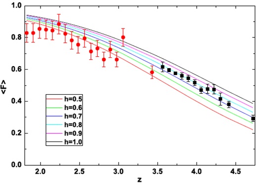
Fig. 1 Mean transmitted flux as a function of redshift for Ωm = 0.23, Ґ = 0.8 x 10⁻¹² s־1, T 0 = 2.5 x 10⁴ K and some selected values of the h parameter. The data points correspond to the Lyα forest measurements obtained by (Rollinde et al. 2013) (red circles) and (Guimarães et al. 2007) (black squares). The color figure can be viewed online.
3. BASIC EQUATIONS
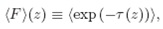
The basic measurement obtained from the Lyα forest is the mean transmitted flux at redshift z defined as
 1
1
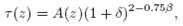
where т(z) is the local optical depth, and angle brackets denote an average over the line of sight. Fol lowing standard methods (Hui & Gnedin 1997), this paper assumes photoionization equilibrium and a power law temperature-density relation, T = T 0 (1 + δ) β , for the low-density IGM, where σ stands for the local overdensity and T 0 for the IGM temperature at mean density (δ = 0). The local optical depth is given by (Peebles 1993; Padmanabhan 2002; Faucher- Giguère et al. 2008a)
 2
2
with
In the expression above, ƒ Lyα. is the oscillator strength of the Lyα transition, v Lyα is its frequency, me and m p are the electron and proton masses respectively, Ωb is the baryon density pa rameter, H(z) is the Hubble parameter, pcrit is the critical density, X and Y are the mass frac tions of hydrogen and helium respectively, which are taken to be 0.75 and 0.25 (Buries et al. 2001), R 0 = 4.2 x 10⁻¹³ cm3 s-1 /(104 K)-0.75, and Ґ is the hydrogen photoionization rate. The effect of redshift-distortions due to thermal broadening and peculiar velocities on the above equations was ne glected since the mean optical depth is in first order independent on these distortions. The mean transmitted flux is a non-linear function of < T >, but the distortions are responsible for only a small effect (Faucher-Giguére et al. 2008b).
The mean transmitted flux is obtained by integrating the local optical depth through a volume density distribution function for the gas Δ ≡ 1 + δ.
 3
3
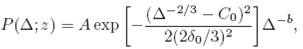
As it is widely known, Miralda-Escudé et al. (2000) derived an approximate analytical functional form for the distribution function given by
 4
4
where the parameters A and Co are derived by requiring the total volume and mass to be normalized to unity. They extrapolated the distribution function and obtained δ0 = 7.61/(1 + z) with an accuracy better than 1%, from fits to a numerical simulation at z =2, 3, and 4 from Miralda-Escude et al. (1996). In order to apply this formalism to our data, the values of b were derived from a cubic interpolation of the values in the simulation. The application of this distribution function to constrain cosmological parameters is well justified, since simulations using different numerical methods and different cosmologies yielded very similar results (Rauch et al. 1997), even though the two simulations share approximately the same amplitude of density fluctuations at the Jeans scale. However, one must be cautious about the limitations of this distribution function. Actually, this function may be affected by several effects. To cite a few: the numerical properties of the simulation, the thermal state of the gas, fluctuations in the UV background, inhomogeneous reionization of hydrogen and helium (Faucher- Giguère et al. 2008b, and references therein).
From now on we will assume a flat ɅCDM cosmology. In this case, the Hubble parameter is given by
 5
5
where we will adopt the convention h = H 0/100 km s -1 Mpc-1 which is the Hubble constant normalized in units of 100 km s-1 Mpc-1.
Figure 1 shows the effects of H 0 on the mean transmitted flux, along with our observational data (red circles) and the data from (Guimarães et al. 2007) (black squares). From our sample we ob tained a scattered data set, compared to the other Lyα sample, which is related to the sample size. It is also evident that our data cover most values of the h parameter; thus, we do not expect tight constraints from the Lyα data set alone.
4. ANALYSIS AND RESULTS
Let us now perform a statistical analysis to find the constraints on the cosmological parame ters. The full set of parameters are represented by p≡(h, Ωm,Ґ, T 0,Ωbh 2, β). We fixed the value of Ω bh 2 = 0.0218 using the latest observations of deuterium (Pettini et al. 2008) from the Big Bang Nu cleosynthesis (Simha & Steigman 2008). We choose β = 0.3 due to the photoheating during Hell reionization (McQuinn et al. 2009), which is expected to occur in the redshifts covered by our samples. An early reionization model with β = 0.62 (Hui & Gnedin 1997) yielded similar results. The posterior probability of the parameters P(p|d) given the data d is
 6
6
where P(d) is a normalization constant, P(p) is the prior over the parameters and P(d|p)∞ e-X2 /2 is the likelihood, using the usual definition. For the Lyα forest data.
 7
7
where {F th}(zi;p) is the theoretical mean transmitted flux, (F)(z i ) is the observational mean transmitted flux and σ (F)(zi) is their respective uncertainty. We treat the combination ҐT0 0.75׳ as a nuisance parameter with a flat prior. The ranges chosen are To = [2, 2.5] x 104 K, from estimates of (Zaldarriaga et al. 2001), and Ґ = [0.8,1] x 10-12 s_1 which cover some measurements reported in the literature (Rauch et al. 1997; McDonald & Miralda-Escudé 2001; Meiksin & White 2004; Tytler et al. 2004; Bolton et al. 2005; Kirkman et al. 2005), although they are in disagreement with the values obtained by (Faucher-Giguère et al. 2008a,b), which used a redshift-dependent relation for T 0 not favoured by our data. We defined the 1, 2 and 3σ confidence intervals as the iso־X 2 re gions given by Δx2 = x2 - x2min equals to 2.3, 6.17 and 11.8, respectively.
It is worth noting that there seems to be a ten sion between the two Lyα samples according to Fig. 1, which shows that the low redshift sample prefers lower values of h. Therefore, we included two parameters to multiply the errors, one for each sample, in order to achieve an acceptable fit. We considered flat priors within the range [1.0,1.1] and marginalized over them.
In what follows, we first consider the Lyα forest data separately, and, then, we present a joint analysis including the BAO signature extracted from the WiggleZ survey (Blake et al. 2012).
4.1 Limits from the Lyα forest data set
Figure 2 shows the results of the statistical analysis performed with the Lyα forest data. The data do not provide good constraints on both parameters. Several sanity checks were performed in order to validate the values obtained in the statistical analysis. The reduced X2 obtained is 0.96. Different values for β, different intervals for ҐT0 0.75 in the marginalization, or even a redshift-dependence for T 0, have resulted in poorer fits compared to what is shown in Figure 2. In addition, even when considering that cosmological constraints are affected by the physical parameters of the IGM, the opposite is also true, that is, that different cosmologies may provide results not compatible with the IGM parameters. In this context, it is recommended to fit cosmological and IGM parameters together in order to obtain more reliable results. The interval for ҐT0 0.75selected in the marginalization, may suffer from a circularity problem, i.e., the values obtained for T o and Ґ were obtained assuming a particular cosmological model. Nonetheless, such parameters should reflect local physics, which are not expected to depend strongly on the assumed model. With this in mind, the effect of a broader interval on the marginalization is a broader interval in the (Ωm, h) plane, but with a well-defined slope. Independent estimates of ҐT0 0.75 are of great interest; F may be determined from the proximity effect (Guimarães et al. 2007; Carswell et al. 1982; Murdoch et al. 1986; Rollinde et al. 2005) and T0 from linewidth measurements, providing an important cross check for the method developed in this work.
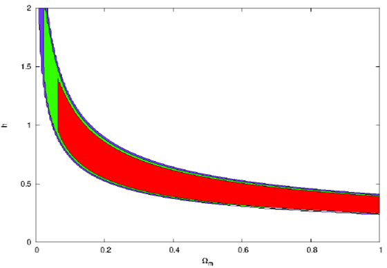
Fig. 2 Confidence regions (68.3%, 95.4% and 99.7%) in the (Ωm, h) plane provided by Lyα forest data. The basic conclusion is that the Lyα forest alone cannot constrain both parameters.
Despite the considerations discussed above, Figure 2 shows that the slope in the (h, Ω m) plane suggests that a joint analysis with an independent test constraining only Ω m could provide interesting limits to the Hubble constant. Thus, a joint analysis with the BAO data is presented in the next subsection.
4.2 The Lyα forest and BAO: A Joint Analysis
In order to obtain better constraints on the cosmic parameters, we performed a joint analysis in volving Lyα forest data and data from baryon acoustic oscillations obtained from the WiggleZ survey (Blake et al. 2012). The BAO scale can be represented by the parameter (Eisenstein 2005)
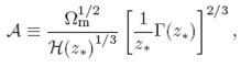 8
8
where z * is the redshift at which the acoustic scale has been measured, H(z) is H(z)/H 0 and Ґ(z *) is the dimensionless comoving distance to z *.
From equation (8), it is seen that the BAO scale is independent of h, and thereby yielded constraints only for the matter density parameter. The statistical analysis was performed with X2 = X2 Lya + X2BAO, where
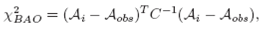 9
9
Ai is a vector of three theoretical values at three effective redshifts, A 0bs is a vector with the respective observed values and C is the covariance matrix for the observations. Here, we used the data provided in Table 2 by (Blake et al. 2012), where we marginalized over all other parameters.
Figure 3 shows the constraints on the pair of parameters (h, Ω m) obtained from our joint analysis involving Lyα forest data and BAO. Within a 68.3% confidence level, we obtained 0.19 ≤ Ω m ≤ 0.23 and 0.53 ≤ h ≤ 0.82. The reduced X 2 is now equals to 1.03. The value for Ω m is lower than what was found by other studies (Amanullah et al. 2010), but is still consistent within the 68.3% confidence level.
Table 1 shows some recent measurements of H 0 using different techniques and data; we can see that our Ho value cannot provide stringent limits that would allow us to make a decision about the correct value of H 0 .The interesting aspect is that the method discussed here provides an additional estimate, independent of the cosmic distance ladder and, covering a redshift range (2 < z < 5), that other techniques cannot provide. Therefore, it is a complementary measurement that can be used as a crosscheck with local and global measurements.

Fig. 3 Contours in the il m - h plane provided by the joint analysis combinig Lyα Forest and BAO. As before, the contours correspond to 68.3%, 95.4% and 99.7% con fidence levels. Note that the best-fit model converges to h = 0.66 and il m = 0.21. These results should be compared with the ones presented in Figure 2.
Table 1 Limits to H 0 from several methods. Rand. Stands for random errors while syst.for systematic errors
| Method | Reference | h |
| Cepheid Variables | (Freedman 2001) (HST Project) | 0.72 + 0.08 |
| Age Redshift | (Jimenez et al. 2003) (SDSS) | 0.69 + 0.12 |
| Age Redshift | (Busti et al. 2014) | 0.649 + 0.042 |
| SNe Ia/Cepheid | (Sandage et al. 2006) | 0.62 ± 0.013(rand.)±0.05(syst.) |
| SZE+BAO | (Cunha et al. 2007) | 0.74 +0.04 -0.03 |
| Old Galaxies + BAO | (Lima et al. 2009) | 0.71+0.04 |
| SNe Ia/Cepheid | (Riess et al. 2009) | 0.742 + 0.036 |
| Time-delay lenses | (Paraficz & Hjorth 2010) | 0.76 + 0.03 |
| CMB | (Komatsu et al. 2011) (WMAP7) | 0.710 + 0.025 |
| SNe Ia/Cepheid | (Riess et al. 2011) | 0.738 + 0.024 |
| Median Statistics | (Chen & Ratra 2011) | 0.680 + 0.028 |
| SZE+BAO | (Holanda et al. 2012) | n 0.74+0.05 -0.04 |
| CMB | (Hinshaw et al. 2013) (WMAP9) | 0.700 + 0.022 |
| SNe Ia/Cepheid | (Freedman et al. 2012) | 0.743 + 0.021 |
| SNe Ia/TRGB | (Tammann & Reindl 2013) | 0.64 ± 0.016(rand.)±0.02(syst.) |
| CMB | (Ade et al. 2014) (Planck) | 0.673 + 0.012 |
5. CONCLUSIONS
In this work, we used a cosmological independent semi-analytical model to describe the IGM and the data from the Lyα forest and baryon acoustic oscillations, in order to constrain cosmological parameters. We provided a cross-check for the Hubble constant H 0 and the matter density parameter Ω m. which were derived by assuming a flat ɅCDM model: we also established that local properties such as F and T0 are only weekly dependent on the adopted cosmology.
We did not obtain good constrains on both parameters from the statistical analysis using only the Lyα forest data. This happened also due to our scarce knowledge about the local properties of the intergalactic medium. However, when we performed a joint analysis involving the Lyα forest data and BAO, we found interesting constraints with the parameters restricted to the intervals 0.19 ≤ Ω m ≤ 0.23 and 0.53 ≤ h ≤ 0.82 within a 68.3% confidence level. All these results are in agreement with recent measurements reported in the literature (Table 1); however, due to the limited sample and our poor knowledge of the IGM, they are weaker. We expect to obtain better and more reliable constraints on the Hubble constant in the near future by using a bigger sample and having a deeper understanding of the IGM (preferably with independent estimates for Ґ and T0. This will make our technique a true complementary of other estimates, with the advantage of being independent of the cosmic distance ladder.

