


Servicios Personalizados
Revista

Articulo
 Inglés (pdf)
 Artículo en XML
 Referencias del artículo
 Enviar artículo por email
Indicadores
 Citado por SciELO
 Links relacionados
-
 Similares en
SciELO
Similares en
SciELO
Compartir

 Permalink
Salud Pública de México
versión impresa ISSN 0036-3634
Salud pública Méx vol.53 no.1 Cuernavaca ene./feb. 2011
ARTÍCULO ORIGINAL
A model for the A(H1N1) epidemic in Mexico, including social isolation
Un modelo para la epidemia de A(H1N1) en México incorporando aislamiento social
Jorge X Velasco-Hernández, Biol, MMat, PhDI, II; Maria Conceicao A Leite, PhD.III
IPrograma de Matemáticas Aplicadas y Computación, Instituto Mexicano del Petróleo. México, DF, México
IIDepartamento de Biociencias e Ingeniería CIIEMAD, Instituto Politécnico Nacional. México DF, México
IIIDepartment of Mathematics, University of Oklahoma. Norman, USA
ABSTRACT
OBJECTIVE: We present a model for the 2009 influenza epidemic in Mexico to describe the observed pattern of the epidemic from March through the end of August (before the onset of the expected winter epidemic) in terms of the reproduction number and social isolation measures.
MATERIAL AND METHODS: The model uses a system of ordinary differential equations. Computer simulations are performed to optimize trajectories as a function of parameters.
RESULTS: We report on the theoretical consequences of social isolation using published estimates of the basic reproduction number. The comparison with actual data provides a reasonable good fit.
CONCLUSIONS: The pattern of the epidemic outbreak in Mexico is characterized by two peaks resulting from the application of very drastic social isolation measures and other prophylactic measures that lasted for about two weeks. Our model is capable of reproducing the observed pattern.
Key words: H1N1; simulation; flu; basic reproduction number; influenza; Mexico
RESUMEN
OBJETIVO: Se presenta un modelo de la epidemia de influenza en México en 2009 para describir el patrón observado desde marzo hasta finales de agosto (antes del inicio de la epidemia invernal), en términos del número reproductivo y las medidas de aislamiento social.
MATERIAL Y MÉTODOS: El modelo es un sistema de ecuaciones diferenciales ordinarias. Se realizaron simulaciones computacionales para la optimización de trayectorias como función de los parámetros.
RESULTADOS: Se exploran las consecuencias de esta última medida combinada con los valores estimados en la literatura médica del número reproductivo básico.
CONCLUSIONES: El patrón de la epidemia mexicana de influenza es bimodal debido a la aplicación del aislamiento social y otras medidas profilácticas que duró aproximadamente dos semanas. Este modelo es capaz de reproducir el patrón observado.
Palabras clave: H1N1; simulación; gripe; número reproductivo básico; influenza; México
Influenza pandemics occur recurrently:1 the Spanish influenza (H1N1 viral subtype) of 1918-1919 killed about 50 million people; the "Asian" influenza (H2N2 viral subtype) appeared in southern China in 1957; the "Hong-Kong" influenza (viral subtype H2N2) appeared in 1968, replaced by a viral reassortant that had the H3HA gene; the "Russian" influenza in 1977-1978 was caused by a viral subtype H1N1 that coexisted with the H3N2 subtype, situation that still persists today, while the reassortant H1N1 and H3N2 produced an H1N2 variant in 2001 that has since disappeared. The explanation for these replacements, or coexistence, is a question that remains to be answered.2
The 2009 influenza epidemic in Mexico was caused by a type A H1N1 virus. It spread rapidly to other areas of the world, with an associated morbidity and mortality that forced the WHO to declare a level five global pandemic alert by late April 2009. In Mexico, health authorities implemented measures to lower the exposure risk and avoid the consequences of contagion, social isolation among them (see Results). These measures were first implemented in the Greater Mexico City Metropolitan Area (GMCMA) and later adopted throughout the country. In the GMCMA, social isolation was declared for about two weeks, with enforced school closures and shutting down all non-essential economic activities for approximately 10 days. These actions were highly controversial because of the high negative impact on the national economy. In this paper we explore the epidemiological consequences of these preventive measures. We use available estimates of the basic reproduction number for influenza (see Results) and data published by the federal Ministry of Health.3 Data from the latter is accumulative for the entire country.
The first outbreak started about the middle of February 2009 in the town of La Gloria in the state of Veracruz.4 Though this site is likely to be the origin of the epidemic in Mexico, it is an isolated small town in the Sierra de Perote and, thus, its weight with respect to the national epidemic which started later is small; therefore it is not included in our study. Our study includes the first five months corresponding to the transient phase before establishment.
The pattern shown by the epidemic consists of a first peak followed in a few weeks by a second larger and broader peak. This scenario raises the questions: Is this pattern the product of the interventions implemented to stop its spread, particularly social isolation? How sensitive is the observed pattern to the value of R0?
One answer may be that the effect of social isolation is to sharply (but not completely) reduce the contact rate between individuals and, consequently, to stop the rise of the outbreak. However, since only a fraction of the population is isolated, once the measure is suspended the epidemic retakes its course and the second peak is produced. Nonetheless, this explanation does not answer the question as to why there was a delay of two months. An answer to this question is not obvious. Once the epidemic starts, the basic reproduction number is fixed. When the outbreak is rising, the second peak should, in principle, depend only on the effectiveness of the isolation. We can thus ask the following: given isolation measures with a certain efficacy, do changes in the value of R0 affect the length of the delay between the first and the second peak? Do different R0's lead to distinct peak sizes?
We introduce a mathematical model for influenza in Mexico to generate the temporal distribution patterns for several different sets of parameter values, which are then used to explain and respond to the questions above. The model uses the SEIR structure for a quasi-stationary population over roughly six months and incorporates a period of social isolation. Notwithstanding this simple hypothesis, the model fits the observed pattern of the epidemic curve up to late August, just before the onset of the expected winter epidemic, at which point it can no longer describe the dynamics. The fit allows us to explore the dynamic pattern as a function of R0. Since factors that characterize this epidemic are important and not well understood -such as Mexico's spatial heterogeneity, seasonality, pre-existing immunity, and interaction with other strains-4,-6 a more detailed model should take into consideration all such inherent complexity.
Material and Methods
This work complies with our institutions' ethical standards; there are no appointed ethics evaluation committees.
Our model is based on a SEIR compartmental scheme and includes compartments for social isolation:

where s,e,y and r represent susceptible, exposed, infectious and immune individuals, respectively. The population has a variable size with recruitment and mortality rates of r and μ. Once the epidemic starts, individuals of each class are isolated into compartments cs, ce, cy and cr at a rate q(t). In this model, q(t) comprises not only the physical isolation that took place in Mexico in April-May 2009, but also other prophylactic measures. The isolation function q(t) has the following form:

where T0 and Tf represent the beginning and end of the isolation period. In Mexico City, the length of physical isolation lasted about 15 days;3 this measure was quickly extended to other cities. Many of the preventive measures taken during isolation lasted much longer and some of them were still functioning several months later. Hence, we assume that individuals suspended sanitary measures at a rate ω.
For completeness, we include a rate for early detection of cases, σ, but we do not elaborate much on its role (see Discussion). This rate represents the detection of exposed but not yet infectious individuals and represents an acceleration in the transition of individuals from the exposed to the recovered class. This is not only an immunological transition but also has a population effect, such that detection implies isolation and treatment of the patient, producing a significant reduction in the probability of contagion; early detection implies treatment with antiviral drugs that effectively reduce infectiousness to zero and contagion to very low levels. For consistency, we assume that the isolation period is longer than the duration of the disease, which comprises the latent time 1/γ and the infectiousness time 1/ε. That is, we have ω < γ + ε, meaning that exposed or infectious individuals in the isolated class cannot leave isolation in said state. Only susceptible and immune individuals leave the isolation class at a rate ω without changing disease state. We formally assume that infections occur within households through contact between susceptible individuals (non-isolated and isolated susceptible) and infectious individuals (non-isolated and isolated). The corresponding rates are denoted by βk and βu, respectively. However, we assume that k >> u, where 0 < u < k < 1. In particular, we take u = 0 and k = 1. The description of the parameters is summarized in Table II. Observe that without isolation and early treatment, the mathematical model reduces to the standard SEIR disease with the basic reproduction number R0= bg / (μ + g)(e + μ). A similar model has been used7 to describe the first month of the epidemic in Mexico City.
Results
On April 16, an epidemiological alert was declared.3 On April 23, a suspension of all educational activities was declared for Mexico City and the State of Mexico and was shortly thereafter extended to the whole country. On April 30, the suspension was extended to all non-essential activities. On May 11, students at the primary educational level returned to classes, followed by students at all other educational levels. Figure 1a shows data on the status of the epidemic on August 15, 2009.
Model parametrization
Table IIb shows the parameters used. Our approach is not concerned with the accuracy of predictions, but rather with the qualitative properties that they share with the actual data. The time to the most recent ancestor, Tmra, in the Mexican republic (Table I) refers to January 11. However, the first reported case in Mexico City occurred around the middle of March. We take the starting date of the epidemic in the country as March 5, close to the upper end of the 95% confidence interval for Tmra, but outside of it (Table I). This choice implies that isolation starts by day 50. Consequently, we set T0= 50 (April 23) in (2). The isolation lasted for about 15 days, equivalent to setting Tf= 65. q0 is the rate at which the population enters isolation once the measure is taken. Seven days passed between the closing of elementary schools (April 23) and the suspension of non-essential activities. This is our estimate for the mean time to isolation.
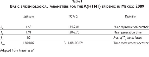
Figure 1b shows the predicted proportion of infected, yr= (y+cy)/N, versus time fixing, R0= 1.85 and q0= 0.17. Our results (Figure 1b) remarkably agree with the data. Based on the official data for August 18, the first confirmed case occurred between March 12 and 19, and the first maximum occurred between April 23 and 30. The second maximum occurred between June 25 and July 2, and the minimum between May 21 and 28. The distance between the midpoints of the two consecutive maxima is about 60 days, and the distance between the first maximum and the minimum is about 26 days. Figure 1b shows the distance between consecutive maxima, about 78 days, and the distance between the first maximum and the minimum, about 31 days (Table IIa).
Dependence on R0
Figure 2 shows curves corresponding to R0= 1.19, 1.46, 1.69, 1.88, all located within the 95% CI (Table I). The rightmost curve is a simple epidemic curve for the lowest R0; the nearest curve to the left of this corresponds to the second value of R0. It is still a curve with a single epidemic peak, but occurring about 250 days (approximately 8 months) after the beginning of the epidemic. The third curve (broken line) corresponds to R0= 1.69. It is no longer an epidemic with a single peak. The effect of the isolation is evident not only in the timing of the epidemic peak, but also in the appearance of a second smaller one. The last curve to the left corresponds to R0= 1.88 and shows the qualitative features of the data for the Mexican case already described above. We therefore conclude that the two-peak pattern -the signature of the Mexican flu epidemic- arises only for certain values of R0 . Those values of R0 are located at the upper third of the 95% CI for the reproduction number (Table I).

Dependence on ω
Our simulations show that 1/ω plays a role in the temporal pattern of the epidemic. This parameter represents the average duration of the prophylactic measures. The baseline value we used is about 16 days, roughly the same duration of the isolation event. Figure 3 shows the predicted disease dynamics for 1/ω = 365, and the same but for 1/ω =180. Shortening the time of use of preventive measures brings the second epidemic peak closer to the first. In Figure 1b, 1/ω = 16 days and the pattern shown closely resembles the observed one, suggesting that the effectiveness of prevention measures lasted an average of 16 days.

Finally, for waning times of 16, 180 and 365 days, for example, the proportion of cases under isolation, cy in (1), produces isolation residence time distributions with increasingly longer tails; therefore, for large t the proportion of cases still protected is highly sensitive to ω.
Numerical explorations for control
Our model shows that the epidemic is produced by the interplay between the rate of isolation, the waning period, and the reproduction number. Now, given the estimated value of R0, what are the parameter values of the "control measures" (β, q0, e) that would minimize the total incidence? To answer this, we minimize the functional:

where y(t) + cy(t) is the total incidence. The discount factor on the integral is a function of mortality, recovery rates, and [ 0,T]. When varying (β, q0, e) while keeping all other parameters constant, we study the following:
fix q0= 0.1, let β in [0.2,0.5] take increments of 0.03, ω in (0,0.1] with increments of 0.01.
fix ω = 0.06, let q0 take increments of 0.1 in (0,1], with β as in case 1.
fix β= 0.5, let ω and q0 as in cases 1 and 2.
Among these choices of triplets (β, q0, e), we are interested in those for which the time series f(t) = y(t)+ cy(t) has two significant maxima in the time interval [0,1000]. Let ƒmax1 , ƒmax2 the first and second maximum of f forward in time. Let ƒmin denote the minimum value of f located between ƒmax1 and ƒmax2.
We define as significant peaks those that satisfy the following: ƒmax i - ƒmin > 1000 for i=1,2. To identify the triplets (β, q0, ω) that lead to two significant maxima we follow the algorithm:
- Integrate (1) for each choice of triplets in cases 1, 2, 3.
- For those triplets with a time series with two significant maxima, compute (3) over [0,1000].
- Obtain the triplet that minimizes (3).
Our results indicate that a minimum occurs for epidemics with general shapes showing a large peak about a year after the first one. For example, for ω=0.06 (fixed), q0= 0.9, β=.32, then tmax 1=50.00, f=2666, tmax 2=355, and f= 1163054; and for ω=0.005, q0= 1 (fixed), β =.32, then tmax 1= 50.00, f=2666, tmax 2=366, and f = 599117. Since (3) is minimized in the former, isolation has to be extremely fast to substantially reduce the impact of the first peak. By isolating individuals fast enough the second peak can be pushed to the window of the next seasonal influenza epidemics.
Discussion
There are several estimates of R0 for influenza. Fraser et al.4 provide the 95% CI (Table I) for the Mexican 2009 epidemic; Chowell et al.10 calculated R0 for the epidemic of San Francisco in 1918-1919 within the range of [2,3]; for the first wave in Geneva in 1918, Chowell et al.11 estimated it in the interval [1.45,1.53]; Boelle, Bernilolon and Desencios12 provided an upper bound in the range of [2.2,3.1] for the Mexican epidemic; Nishiura et al.13 provided the interval [2,2.6] for Japan; Massad et al.14 estimated it at 2.68 for the flu epidemic in Sao Paulo of 1918; Mills et al.15 estimated the reproduction number for the 1918 pandemic at under 3. The estimates for Mexico have a broad interval. Our model suggests that R0 for this epidemic must be at the upper end of the confidence interval identified by Fraser et al.4
R0 estimation is highly sensitive to the generation time and, necessarily, there is a high variability in the duration of its latent 1/γ and infectious 1/ε periods.16 For H1N1, the CDC reports a latent period ranging from 1 to 7 days, with 1 to 4 being more likely, and an infectious period up to 7 or 10 days. Using published estimates, we conclude that if parameters are fixed at their baseline values (Table IIb) and we vary R0 then for values below 1.7 the simulations of (1) are not consistent with the pattern shown in Figure 1b. This suggests that, for the Mexican epidemic, the lower bound for R0 is around 1.7.
The basic SEIR model shows only one epidemic peak. Thus, the second peak observed in our simulations is the original epidemic, delayed by the action of isolation. This effect has already been reported by Epstein, Parker et al.17 and Cayley, Philp et al.18 but in different contexts. Here, where we model the application of social distancing, the delay between the two observed peaks is not only a function of the length of the isolation time but also a function of R0 , ω and q0. We show that shortening the waning time 1/ω would bring the second epidemic peak closer to the first (Figure 2).
Figure 1b shows a close resemblance to the observed pattern when 1/ω = 16 days, suggesting that the effectiveness of prevention measures lasted about 16 days. The numerical explorations described reveal that if isolation is implemented fast enough, (q0 close to one), the second peak will be delayed approximately one year, allowing for time to take preventive actions before the seasonal influenza epidemics outbreak.
Conclussions
The epidemic outbreak in Mexico shows two peaks resulting from the application of drastic social isolation and other prophylactic measures that lasted at least two weeks. We reproduced this pattern, showing that it only occurs within a relatively narrow range of values for crucial parameters, such as the basic reproduction number, the isolation rate and the waning of prevention measures. Significant qualitative changes in this pattern obtained through manipulation of these parameters generated delayed single-peak epidemics appearing many weeks after the end of the isolation period, or two-peaked epidemics but with much greater delay between them.
Mexico is a large country and the influenza epidemic occurred in geographically distant and different regions. From the patterns of influenza dispersal reported,21 the virus spread from Mexico City and other cities (San Luis Potosi, Zacatecas, etc) to other population centers via public transportation (mainly bus or plane), and from there to smaller communities. While the data reported by the federal Ministry of Health lumps together such geographical complexity, since social isolation and other measures were implemented across the whole country, their effect on local epidemics was likely the same as that observed at the country level, as our model shows. The model incorporates a minimal amount of information that can reproduce the observed pattern using only known parameters and excluding treatment.
While our objective has been to explain the bimodal disease, there are certainly other factors that our model neglects, such as the effect of space and of asymptomatic infections; nevertheless, we assert that such factors do not play a role in explaining the two-peaked epidemic. In addition, we do not have sufficient information to parameterize such an elaborate model.
A third epidemic peak started in Mexico in late September. The initial appearance of an epidemic peak after August 11 is a feature not predicted by our model and represents a true second wave of influenza -a mixture of seasonal and H1N1 viruses.
Finally, surveillance for detection occurs at rate σ and is set as 0 in this work. This was certainly not the case in the Mexican epidemic but, unfortunately, early detection was poor. Fajardo-Dolci et al.19 report that only 17% of cases received medical attention within the first 72 hours from the onset of symptoms, concluding that delay in treatment and medical attention were significant factors for the magnitude of the mortality rate. Similar conclusions are reported by Grijalva, Talavera, Solorzano et al.20 Thus our estimate of σ= 0 , while inexact, is still a reasonable first approximation.
Acknowledgments
We would like to thank Suzanne Lenhart and Zhilan Feng for their helpful discussions. We also acknowledge funding from NIMBioS (National Science Foundation grant EF-0832-858).
Declaration of conflicts of interest: The authors declare that they have no conflict of interests.
The authors declare that they have no conflict of interests.
References
1. Neumann G, Noda T, Kawaoka Y. Emergence and pandemic potential of swine-origin H1N1 influenza virus. Nature 2009;459:931-939. [ Links ]
2. Earn DJD, Dushoff J, Levin SA. Ecology and evolution of the flu. TRENDS in Ecology and Evolution 2002;17:334-340. [ Links ]
3. Ministry of Health. Estadísticas de la epidemia. Influenza A(H1N1). Mexico: Ministry of Health, 2009. [Accessed on August 21, 2009]Available at: http://portal.salud.gob.mx/contenidos/noticias/influenza/estadisticas.html [ Links ]
4. Fraser C, Donnelly CA, Cauchemez S, Hange WP, Van Kerkhove MD, Hollingsworth TD, et al. Pandemic potential of a strain of influenza A (H1N1): early findings. Science 2009;324(5934):1557-1561. [ Links ]
5. Cohen J. Past pandemics provide mixed clues to H1N1's next moves. Science 2009;324:996-997. [ Links ]
6. Park AW, Glass K. Dynamic patterns of avian and human influenza in east and southeast Asia. Lancet Infect Dis 2007;7(8):543-548. [ Links ]
7. Cruz-Pacheco G, Duran L, Esteva L, Minzoni AA, López-Cervantes L, Panayotaros P, et al. Modelling of the influenza A(H1N1)V outbreak in Mexico City, April-May 2009, with control sanitary measures. Euro Surveill 2009;14 (2). [ Links ]
8. Tuite AR, Greer AL, Whelan M, et al. Estimated epidemiologic parameters and morbidity associated with pandemic H1N1 influenza. CMAJ 2009;182(2):131-136. [ Links ]
9. Pourbohloul B, Ahued A, Davoudi B, Meza R, Meyers LA, Skowronski DM, et al. Initial Human Transmission Dynamics of the Pandemic (H1N1) 2009 Virus In North America : Methods. Influenza Resp Viruses 2009;3(5):215-222. [ Links ]
10. Chowell G, Nishiura H, Bettencourt LMA. Comparative estimation of the reproduction number for pandemic influenza from daily case notification data. J R Soc Interface 2007;4(12):155-166. [ Links ]
11. Chowell G, Ammon CE, Hengartner NW, Hyman JM. Transmission dynamics of the great influenza pandemic of 1918 in Geneva, Switzerland: assessing the effects of hypothetical interventions. J Theor Biol 2006;241:193-204. [ Links ]
12. Boelle PY, Bernillon P, Desenclos JC. A preliminary estimation of the reproduction ratio for new influenza A(H1N1) from the outbreak in Mexico, March-April 2009. Euro Surveill 2009;14:10-13. [ Links ]
13. Nishiura H, Castillo-Chavez C, Safan M, Chowell G. Transmission potential of the new influenza A(H1N1) virus and its age-specificity in Japan. Euro Surveill 2009;14(22):pii=19227. [ Links ]
14. Massad E, Burattini MN, Coutinho FAB, Lopez LF. The 1918 influenza A epidemic in the city of São Paulo, Brazil. Med Hypotheses 2007;68(2):442-445. [ Links ]
15. Mills CE, Robins JM, Lipsitch M. Transmissibility of the 1918 pandemic influenza. Nature 2004;432:904-906. [ Links ]
16. Lessler J, Reich NG, Brookmeyer R, Perl TM, Nelson KE, Cummings DA. Incubation periods of acute respiratory viral infections: a systematic review. Lancet Infect Dis 2009;9:291-300. [ Links ]
17. Epstein JM, Parker J, Cummings D, Hammond RA. Coupled contagion dynamics of fear and disease: mathematical and computational explorations. PLoS ONE 2008;3(12):e3955. [ Links ]
18. Caley P, Philp DJ, McCracken K. Quantifying social distancing arising from pandemic influenza. J R Soc Interface 2005;5:631-639. [ Links ]
19. Fajardo-Dolci G, Hernandez-Torres F, Santacruz-Varela J, Rodríguez-Suárez J, Lamy P, et al. Perfil epidemilógico de la mortalidad por influenza humana A (H1N1) en México. Salud Publica Mex 2009;51(5):361-371. [ Links ]
20. Grijalva-Otero I, Talavera JO, Solorzano-Santos F, et al. Critical analysis of deaths due to atypical pneumonia during the onset of the influenza A(H1N1) virus pandemic. Arch Med Res 2009;40(8):662-668. [ Links ]
 Address reprint requests to:
Dr. Jorge X. Velasco
Programa de Matemáticas Aplicadas y Computación
Instituto Mexicano del Petróleo
Eje Central Lázaro Cárdenas 152
San Bartolo Atepehuacan. 07730, México DF
E-mail: jx.velasco@gmail.com
Received on: March 4, 2010
Accepted on: September 29, 2010

