1. Introduction

Electric gas discharges are carried out in many applications of industry and science. Glow discharge plasmas are considered cold even when they reach a mean temperature of approximately 11,600 K. Many weakly ionized laboratory plasmas are classified as low temperature plasmas [¹,²]. Some of the most well-known technological applications that use cold plasmas are fluorescent luminaries (neon, mercury, etc.). Another application of plasma technology can be found in food industry, where the sterilization processes of a wide variety of vegetables are plasma-based at low temperatures [³]. Plasma technology is also used to sterilize thermolabile equipment and laboratory instruments that are sensitive to humidity [⁴]. However, some developments are so far limited by the poor knowledge of some of the basic properties of plasma. The inherent non-linear dynamics of plasma makes it difficult to describe [⁵]. Currently, glow discharges in different types of gases, subject to stationary electric and magnetic fields and temperature conditions, are under theoretical and experimental investigation with the aim of determining the spatial distribution of all charged and uncharged particle involved.

There is no single way to approach plasma modelling. A plasma is a system containing a very large amount of particles, usually of the order of Avogadro’s number, which makes the description of individual particles hopeless. A common theoretical tool for plasma characterization is the macroscopic (fluid) approximation, which is the easiest option for cold plasma modelling. Evidence suggests that most macroscopic mathematical models for cold plasmas can be derived by considering all the involved species as fluids. This is a reasonable assumption if we consider a pressure range within 0.5 to 5 Torr [⁶]. These approaches for plasmas are valid if, for instance, the driving frequency of a radio-frequency (RF) discharge and the discharge gap are much larger than the electron energy relaxation time (of the order of nano seconds) and the mean free path (of the order of tens of μm), respectively, making the fluid model suitable to be used in this regime [⁷].

It is well known that all available computational methods allow to consider diverse phenomena as, for instance, particle collisions and interactions, excitation, and recombination. Additionally, the use of numerical tools enables a proper handling of non-linearities, resulting in a more complete characterization of plasma dynamics [¹]. Nevertheless, the theoretical problem of predicting plasma physics is not only reduced to the use of numerical tools, but can be addressed via analytical methods, whose capability to represent the physics of cold plasmas is highly appreciated in literature. Analytical solutions for cold plasma models have a reputation for being too complicated, mainly due to cumbersome boundary conditions and non-linearities which lead to oversimplifications [⁸], that in most cases reduce the underlying problem to a set of diffusion equations [⁹]. However, there are advantageous physical situations that can be genuinely described by specific analytical solutions that cover most of the phenomena associated with such special cases. The latter, motivates the proposal to study basic but interesting cases of plasma physics which could be analysed with analytical tools. In our case, we use an analytical method that can be applied to model a wide range of cold plasma problems, with its specific physical assumptions, while taking into account phenomena such as recombination, attachment, and ionization. The proposed solution approaches the non-linear mathematical nature of a glow discharge by asymptotic expansions, which not only involve particle interactions but the advantage of non-linear effects to study three different geometrical configurations of electrodes: a pair of flat plates, a pair of concentric cylinders, and a pair of concentric spheres. With most of the cold plasma reactors developed in complex geometries, we consider the effect of cavity geometry in the behaviour of cold plasmas. In fact, a simple pair of coaxial cylindrical electrodes are directly applicable to the treatment of superconductive cavities, supersonic nozzles and particle accelerators, processes which imply the removal of chemical impurities that lead to electric losses or unfavorable hydrodynamic turbulence [¹⁰]. In order to estimate the predictive capabilities of the analytical method, we compare the analytical solutions with numerical calculations obtained through a high-order spectral method based on Chebyshev polynomials.

2. Physical model

The glow discharge in an inert monatomic gas is modelled under electrostatic DC configuration for three different geometrical cavities depicted in Fig. 1. The cavities are designed in such a way that the bounding walls act as the driving and ground electrodes, so that an electric potential can be applied through the walls in order to ionize the gas bounded inside the cavities. The electric connections in Fig. 1 are regularly used in sputtering applications, where a negative voltage is applied to the cathode while the anode is grounded, commonly referred as cathodic sputtering [¹¹]. The chamber where a discharge is performed often plays the role of the anode, assuming a zero potential in its surface. The first configuration, (Fig. 1a), consists of two flat plate paralell electrodes, the second configuration, (Fig. 1b), consists of two concentric cylindrical electrodes, where the outer one is a hollow cylinder and the inner one is a solid cylindrical rod. The third configuration, (Fig. 1c), consists of two concentric spherical electrodes, where the outer one is a hollow sphere and the inner sphere is solid. Notice that in all three cases, the region where the gas is ionized corresponds to the gap going from a to b, which is the distance separating the electrodes.

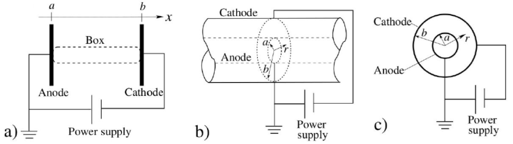
Figure 1 Sketch for the three arrays of cavities in which the glow discharge was modelled. a) Parallel flat electrodes. b) Concentric cylinders. c) Concentric spheres. For all the cases the non-powered anode was the grounded electrode. 

Once a constant gas flow reaches a stationary distribution inside the space between the electrodes, the powered electrodes reach the breakdown potential to ionize the monatomic gas. We assume that the ionization is obtained by collisions of electrons with neutral gas atoms, reaching the removal of only one electron in each collision. The creation of negative ions is neglected since only positive ions and free electrons are considered in the plasma dynamics. We do not consider any applied or induced magnetic field, thus magnetohydrodynamic effects are safely neglected. The recombination rate is considered constant and its contribution to the overall process is considered to be negligible. Furthermore, it is assumed that positive ions generated from collisions exchange energy through elastic collisions, and therefore are assumed to be at the same temperature as neutral species. The ion mobility and diffusivity coefficients are considered constant. Finally, we consider that at the macroscopic scale, as well as, the electron’s and ion’s mean temperatures are constants, so bulk gas convective motion is negligible. Our main aim is to characterize the plasma, in terms of the electric potential, electric field and spatial density distributions of positive and negative charges for each analysed geometry. Taking into account all these assumptions, the mathematical model is presented in the next section.

3. Mathematical model

The cold plasma is modelled with the fluid approximation expressed in the following equations

Where Eqs. (1) and (2) are balance equations for electrons and ions densities n _e and n _i , while J _e and J _i are the electron and ion fluxes. Equation (3) is the Poisson’s equation for the electric potential, ϕ, associated with the self-consistent electric field, resulting from the distributions n _e and n _i [⁶]. Here e is the electron’s charge and 𝜖 is the electric permittivity of the medium. The source term k _i considers the reaction rate (i.e. ionization only due to collisions of electrons with neutral gas atoms) occurring inside the chamber and is expressed as

Where k _io is known as the pre-exponential factor of the reaction rate [¹²]. The Boltzmann constant, the electron temperature in K, the neutral particle concentration in the plasma, and the reaction activation energy are denoted by k, T _e , N and E _i , respectively. The particle fluxes of electrons and ions are given by

respectively, where µ _i and µ _e are the mobilities of ions and electrons, respectively, and D _i and D _e are the corresponding diffusion coefficients. E→ is the total electric field which is calculated from

Equations (1)-(7) form a closed system which describes the glow discharge of cold plasmas that satisfies the boundary conditions described below.

4. Asymptotic solution

Assuming that the rate of ionization k _i inside the plasma is small, the Damkohler number can be considered as a small parameter, allowing the one-dimensional cold plasma model to be solved by asymptotic expansions for the three geometries shown in Fig. 1. The method of solution is described in this section with general assumptions. It is convenient to stress here that we try to model DC ionization assuming that the system remains in steady state and that the phenomenon is one-dimensional. We look for asymptotic solutions for n _e , n _i and ϕ expressed as perturbation expansions in the small parameter D _a , that is,

where the superindex denotes the order of each term in the approximation. The symbol O(Da4) represents all terms of order Da4 and higher that are neglected in Eqs. (24)-(26). We now propose the final approximation by writing the term of ionization as follows:

By substitution of (24)-(27) into Eqs. (15)-(17) the solutions for n _e , n _i , and φ that satisfy boundary conditions (18)-(23) can be obtained to the considered order. The explicit analytic expression of the solutions for n _e , n _i , and φ for the flat parallel electrodes geometry are presented in the Appendix. Lastly, we note the approximate contribution of each order to the general solution. The first order terms proportional to O(Da) contributes 99.967 % of the solution. Terms of ODa2 contributes approximately 0.032 %, while the contribution of ODa3 is three orders of magnitude smaller. Even though the second and third order contributions become numerically insignificant to our analytical solution, there is justification to keep them. First of all, the first-order conditions seemed to be incomplete in mathematical terms. Furthermore, adding the ODa2 term, the solutions near the boundaries were qualitatively improved. The ODa3 term is comprised in our solution just for illustration purposes and due to the ease of its calculation.

5. Numerical solution

A Chebyshev spectral collocation method (CSCM) was used to obtain a numerical solution for the cold plasma model defined by Eqs. (15)-(17). The details of CSCM can be found in the specialized literature [¹³-¹⁶]. Let us consider the Chebyshev approximation of n _e (x), n _i (x), φ(x) defined in a one dimensional rectilinear coordinate for x ∈ [-1,1] as

where the upper index (e), (i) and (φ) stands for the Chebyshev polynomials and the coefficients for electron density, ion density and electric potential, respectively. The order of approximation is denoted by N. The differential equations are satisfied at certain points called the Gauss-Lobatto collocation points, represented as

In the case of the cylindrical, spherical and even with rectilinear coordinates, we use a mapping of any arbitrary interval r ∈ [R ₁, R ₂] to standard interval x ∈ [-1,1], which is needed to fit the requirement of Chebyshev polynomials, that is,

Derivatives are thus treated as

6. Results

6.1 Linear regime

In this section, we present the results obtained from the mathematical model in the linear regime, where the dimensionless parameters P_e, P_i, Γ, γ, and β take values less or equal to unity. Results of the analytical procedure are compared against results from the numerical method in Fig. 2. Since analytically is not possible to consider Neumann boundary conditions on both boundaries, the boundary condition of ion density at the cathode (20) was replaced by the expression n _i = ni _c = 0.6. Such value is actually the one obtained in numerical calculations when we apply Neumann boundary conditions (20) and (23). The dimensionless parameters in this regime, used for the whole set of electrodes were: Da=3.3×10-4,Γ=10-2,β=10-2, γ=10-2, Pe=10-2, Pi=1 and the values for the potential were φ = -1 and φ = 0, at the cathode and the anode, respectively. These parameters fulfill the requirement of a linear regime. Finally, the parallel set of flat electrodes were positioned at a = 0 and b = 1. In turn, both the cylindrical and spherical electrodes were positioned at a = 0.085 and b = 1.

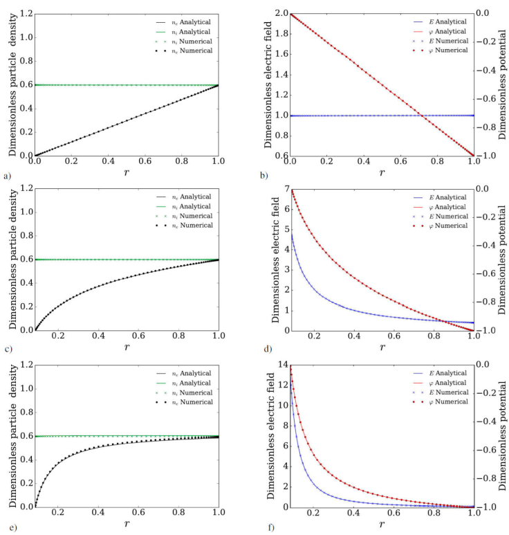
Figure 2 Electron density, ion density, potential and electric field profiles. Linear regime. First row: Parallel flat plates. Second row: Concentric cylinders. Third row: Concentric spheres. Continuous lines: Analytical model. Symbols: Numerical solutions. 

Figure 2 shows an excellent comparison between the analytical and numerical results for the three geometrical configurations of electrodes. At this point we can show that our numerical and analytical tools are mathematically consistent with each other. Therefore, we can emphasize the distinct distribution of particles and fields within each pair electrodes. This is mainly due to the difference in surface area of each pair of electrodes. Evidently, if the surface electric charge is measured in an arbitrary position at the same distance from the anode or the cathode in each system, different values will be obtained. Therefore, it appears that the accumulation or absence of charge in these surfaces is abruptly modified from one geometry to the other. This is clearly illustrated in the behavior of the electric field and the electric potential near the anode, namely, in the Figs. 2b, 2d and 2f. Since all results were obtained with the same values of the transport coefficients, it can be stated that geometry takes a relevant role (perhaps the most important) in the distribution of potential, electric field, and of course particles. This is confirmed by the agreement of both methods of solution. The availability of the analytical solutions in the linear regime allows for the validation of numerical models of cold plasmas.

6.2 Non-linear regime

In this section we present the comparison of asymptotic and numerical results of the model formulated by Eqs.(15)-(17) for a cold plasma in the non-linear regime, which inherently implies large values of P _e ~ 10² and P _i ~ 10³ using common discharge conditions in Argon. These conditions imply that drift process becomes relevant, and diffusion, although not negligible, is not the only process involved. There is also a relevant fact about the value of β ~ 10⁴ which implies that electron diffusion is many orders of magnitude larger than ion diffusion. Lastly, the parameter Γ indicates the magnitude of the inverse potential. It is important to highlight that the requirements that makes the analytical solution mathematically valid are not fulfilled in this regime, but for the sake of comparison, they are also obtained to show their limitations. Finally, it turns out that the trends of the analytical solutions are very similar to those obtained with numerical calculations.

In Fig. 3a), we observe that ion and electron distributions resemble bell-shaped curves. In addition, the peak of ion and electron density are approximately 1.62 and 1.49, respectively, for asymptotic results, while for numerical results, these peaks were found at 1.38 and 1.35, respectively. We can observe that in the non-linear regime, only a qualitative agreement between the analytical and the numerical solutions is obtained. These theoretical results present qualitative similarities with solutions obtained in the literature with different numerical methods [¹⁷-¹⁹]. Notice that the ion densities at the powered electrode (r = 1) present different boundary conditions in the numerical solution with respect to the analytical one. This is due to the fact that in the numerical solution we used Neumann conditions (20) and (23), being easy to implement in both electrodes, whereas analytically this is not easily accomplished, and n _i = 0 was imposed instead of (20) at the cathode for the analytical solution.

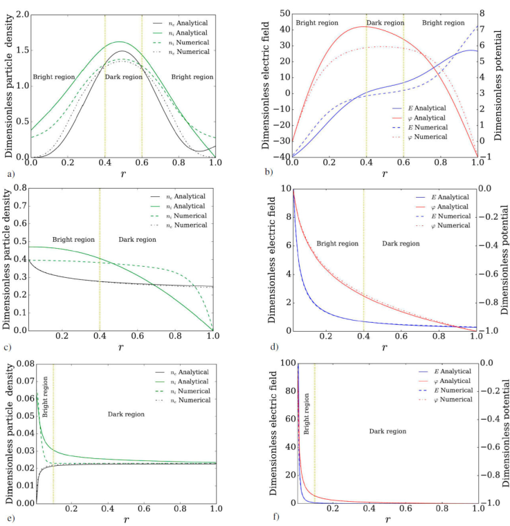
Figure 3 Electron density, ion density, potential and electric field profiles. Non-linear regime. First row: Parallel flat plates. Second row: Concentric cylinders. Third row: Concentric spheres. Continuous lines: Analytical model. Symbols: Numerical solutions. 

It is important to remark that the parameters were different for the numerical and the analytical results. The parameters used in the numerical calculations were Da=5.5×10-5,Γ=488.9, β=104, γ=0.046, Pe=0.9, Pi=900. The parameters used in the analytical calculations were Da=5.5×10-4, Γ=200, β=104, γ=0.046, Pe=25, Pi=0.15. The choice of the latter dimensionless values in the analytical solutions is due to the fact that they yield results qualitatively similar to the numerical ones. For the other set of electrodes such values were obtained by trial and error considering them as an estimate of those used in the numerical solutions. Figure 3b) shows the potential and electric field distributions for the flat plate electrodes configuration. The electric charge of the plasma is predominantly positive in most of the gap between electrodes. The potential satisfies the boundary conditions imposed, which are φ = -1 at the cathode and φ = 0 at the grounded electrode.

The stationary distributions of ions and electrons for the case of cylindrical electrodes are shown in Fig. 3c) along with the electric field and electric potential distributions in Fig. 3d). The analytical solution shown in Fig. 3c) qualitatively reproduces many features of the numerical solution except for n _i . The value of the parameters used in the numerical calculations were Da=60×10-6, Γ=1, β=103, γ=0.022, Pe=0.5, Pi=40. In turn, the parameters used in the analytical calculations were Da=60×10-6,Γ=0.01, β=103, γ=0.022, Pe=0.5, Pi=40. The values of the parameters used for the numerical solution were estimated from those used in the literature. Therefore, distributions of particle density and electric fields are comparable to results reported experimentally and numerically [²⁰]. It is worth noting that the behaviour of our system was disturbed with a low level of drift of electrons, leaving diffusion to become the most relevant transport mechanism. In the case of ion transport, drift is the most important phenomenon in the core of the plasma. Finally, in Fig. 3d) we can observe a similar slow decay in the potential as well as in the electric field along the space between electrodes, but much sharper in the latter.

Figure 3e) shows ion and electron distributions for the concentric spheres case, where a predominantly positive plasma can be observed near the inner electrode. The complete set of boundary conditions are (19)-(23) with a modification for the ion density at the anode in Eq. (23), used for both the analytical and the numerical solutions, namely, J _i = J _A at r = 0.006. Results and boundary conditions presented here are an attempt to qualitatively reproduce results reported in a specific work [²¹]. Here, J _A is a specific value of electric current which could be measured in the anode, but we choosed J _A = -10. However, for both numerical and analytical solutions, the ion density takes a positive value in the cathode at r = 1 as a result of an imposed Dirichlet condition, which implies the modification of condition (20) into n _i = 0.024. The parameters used in the numerical model were Da=40×10-5,Γ=1, β=102, γ=0.01, Pe=0.09, Pi=10 and for the analytical solutions, Da=40×10-5, Γ=0.1, β=10, γ=0.001, Pe=0.001, Pi=96. In this specific set of electrodes we observe a difference between the analytical and numerical results for the ion density. However, as seen in Fig. 3f), there exists a case of the distribution of the electric field and potential where the profiles of the numerical and analytical solution are very similar.

The results presented in Fig. 3e) indicate that the case of two concentric spherical electrodes is mainly characterized by a considerable increase of the concentration of charged particles in the anode region, especially of the positive species. While the glow discharge in flat geometry Fig. 3b) is characterized by a smooth behaviour of potential and electric field in most of the discharge gap, an abrupt drop in potential in the glow discharge is observed in the spherical and cylindrical geometries.

Experimental observations of the glow discharges between parallel electrodes [²²] and cylindrical electrodes (hollow cathode) [²³] show the generation of luminous and dark regions within the plasma. In order to contrast the experimental observations with our results, the yellow dotted vertical lines in Fig. 3 delimit the bright and dark regions within the plasma. In the parallel electrodes configuration, first row in Fig. 3), the electric field magnitude is low between r = 0.4 and r = 0.6, which denotes a dark region (or Faraday dark space). Outside the latter region, the electric field magnitude is increased, which promotes two bright regions denoted as anode and cathode glow. For the cylindrical electrodes, second row in Fig. 3, we can only identify two regions, the anode glow close to the inner electrode due to the increase in particle density and electric field magnitude, and the dark one which covers most of the system. A similar distribution of the bright and the dark regions can be appreciated for the concentric spheres case, third row in Fig. 3, however in this case the anode glow is shorter than the previous case (concentric cylinders) due to the abrupt decay of the electric field in the r-direction. We must note that, the physics of a DC glow discharge is more complex than our theoretical approach which only reproduces some qualitative aspects of real glow discharges because of the strongly restrictive assumptions. However, these asymptotic solutions represent a simple useful tool to understand some basic aspects of DC glow discharges.

7. Concluding Remarks

Analytical and numerical solutions for a non-linear mathematical model of a cold plasma were found for different electrode configurations. A glow discharge was achieved by ionization of an inert gas with an applied electric field between the gap of three different configurations of electrode pairs. Analyzed configurations correspond to parallel plate, concentric cylindrical and concentric spherical electrodes. With the aim of determining electron and ion densities as well as potential an electric field distributions, asymptotic expansions were implemented to solve the plasma model analytically with power series in terms of the Damkohler number, that were truncated up to third order to make the problem manageable.

Regarding the comparison with the available numerical results, the analytical solutions are strongly limited by boundary conditions and the asymptotic approximation. Nevertheless, we developed a numerical tool based on a spectral method to solve the complete set of equations of the cold plasma model. By maintaining the dimensionless parameters within a given range, it was possible to exactly match the numerical and the analytical results in the three electrode configurations. Thus, the theoretical scope of the present work is limited by the values with which the dimensionless parameters can achieve coinciding numerical and analytical results.

We found that our analytical and numerical results agree qualitatively in the non-linear regime as compared with results found in literature. Nonetheless, given to the scarcity of exact solutions in the literature our asymptotic solution in the linear regime is useful for the validation of numerical models for cold plasma with the specific assumptions mentioned in this work.