


 nueva página del texto (beta)
 Inglés (pdf)
 Artículo en XML
 Referencias del artículo
 Enviar artículo por email
 Citado por SciELO
  Similares en
SciELO
Similares en
SciELO 
 Permalink
1. Introduction
The development of new magnetic nanomaterials has gained much importance due to their novel applications in several disciplines, mainly those related to biomedical applications1.
Currently, iron oxide magnetic nanoparticles (MNPs) of magnetite are manufactured following various chemical methods2,3, obtaining beads with spherical shape and core-shell structures, which have high magnetic saturation, low hysteresis, and good biocompatibility with cell cultures1,4. The theoretical modeling of the MNPs allows us to study the magnetic behavior of these nanomaterials under different thermodynamic conditions, also to quantify the interaction between nanoparticles to determine the magnetic anisotropic effects involved5.
The ferrimagnetic behavior of magnetite and a lot of ferrites was widely explained by Louis Néel during the 20th century. In magnetite, this response is caused by the tetrahedral and octahedral overlapped sublattices of the ions Fe3+ and Fe2+/Fe3+, which are located in the interstitial places of the crystalline structure FCC formed by the oxygen atoms, where the antiparallel orientation of the magnetic moments are arranged as an “antiferromagnetic imperfect ordering6”. The antiferromagnetic and ferrimagnetic orderings depend on the temperature T and both disappear above a critical temperature TN or TC (called Néel or Curie temperature, respectively), reaching a paramagnetic behavior6,7.
Monte Carlo (MC) computer simulations are a useful alternative to complement the analysis of the magnetic properties of the MNPs; several works have modeled the magnetization M of antiferromagnetic systems based on iron oxides (or magnetic systems in general) employing the Ising model8-10. Other works have used MC computer simulations with similar purposes, but using an oversimplified model, which considers a fluid of magnetic hard spheres (MHS) or discs, which are influenced by a magnetic field of magnitude H11,12.
The main aim of this work is to study both experimentally and theoretically the magnetization (M) behavior of magnetic core-shell spheres (CSS), with a particular interest in CSS of magnetite coated with dopamine. This type of nanoparticles has been probed successfully in vitro and in vivo experiments of magnetic hyperthermia. The molecular approach here considered to carry out MC computer simulations is explicitly built with the measured parameters of the CSS, such as the diameter of the magnetic core, thickness of the coating, magnetic moment, concentration of MNPs, magnetic field, anisotropy constant, and temperature. Later, the computed magnetization dependences M vs H and M vs T are analyzed and compared with those obtained using a vibrating sample magnetometer (VSM).
Thus, by combining MC computer simulations and analytical approximations for the magnetization, using some physical parameters about the composition and magnetic moment of the CSS, it is possible to reach a better understanding of their magnetic properties in a wide interval of temperatures. Our main hypothesis is that the main mechanisms of magnetization can be accounted for by considering explicitly the excluded volume interaction, the dipole-dipole interaction between the coated nanoparticles, the external magnetic field, and the anisotropic magnetic contribution.
2. Theoretical background
2.1. Potential model
To carry out the computer simulations of the magnetic CSS, we consider a simplified fluid composed of N spheres of diameter σ (magnetic hard-spheres; MHS) of volume Vi within a volume V at a temperature T. The MHS can be oriented by an external magnetic field B following the Zeeman energy law, since each sphere has an intrinsic dipolar moment μi. Therefore, dipole-dipole interactions between MHS should be taken into account. Additionally, the uniaxial anisotropy energy of the CSS is explicitly considered by introducing its magnetic anisotropy constant ki and the orientation of the anisotropy along the
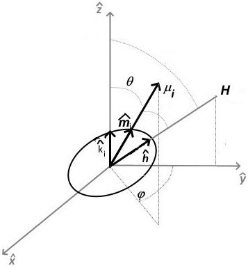
Figure 1 The coordinate system and all the vectors and angles with the origin in the geometric center of a CSS.
The Hamiltonian of the dipolar fluid is given by,
where K is the kinetic energy and Vhs represents the typical hard-sphere repulsive interaction at short distances13.
2.2. Monte Carlo computer simulations
The Monte Carlo computer simulations are carried out in the canonical ensemble with N = 512 particles using the standard Metropolis criterion11 with an acceptance ratio of 30%. 106 MC steps are used for equilibration and another 106 MC steps to gather statistics; each MC consists of either a displacement or a rotation. In the simulations, the values of B are modified to sweep a set of intensities simulating the operation of a VSM11,13. A similar procedure is followed to compute the dependence M vs T; B = (0 H is fixed and a sweep of temperatures is programmed; at each temperature, equilibration is reached. Magnetization is computed according to the following Eq. (2), where <…> denotes an ensemble average.
2.3 Analytical approximation
The magnitude of the magnetization of paramagnetic and superparamagnetic MHS with anisotropy energy negligible is well described by the Langevin expression (Eq. (3)), with kB being the Boltzmann constant.
Nevertheless, when the anisotropy energy and dipolar contributions of the MHS become significant, the expression for M must be modified. Initially, the dipolar interactions can be expressed in terms of a coupling factor
Then, the potential energy U weighted with the thermal energy is rewritten as Eq. (5).
In Eq. (5), the free (Efree) and dipolar coupling (Edip) energy densities are separated as follows in Eq. (6), with
The component of the magnetization aligned with H can be calculated as the expectation value 〈M〉 = ∫ d(MP, where the Boltzmann probability distribution P can be expanded (considering weak dipolar interactions) in powers of λβ = λ/kB T as P = Pfree (1 + λβF (
For the calculation of 〈M〉free, it is suitable to take Vi = Vmean as the mean volume of the particle size distribution and also κi = κmean corresponds to the mean uniaxial anisotropic constant, allowing the determination of 〈M〉free as the average of the monodisperse ensemble magnetization
In the same way, the partition function of a monodisperse system within the canonical ensemble can be calculated in spherical coordinates as
As shown by several authors17-19, Zfree can be expressed as a single integral (see Eq. (9a) below) in terms of the modified Bessel function of zero-order I0 for exact numeric calculations, or as a series expansion of Eq. (9b).
Analyzing the limits of low and high amplitudes of H, it is possible to compute the reduced magnetization of the free particles (corresponding to ƒ(σi) = 1) obtaining Eq. 9(c).
Expanding Eq. (9b) for low and high amplitudes of H, and calculating Eq. (9c) up to second-order in the reduced anisotropy (, and considering
With these approximations for
2.4. Layer thickness
The thickness Δ of the coating material joined to a spherical nanoparticle (called core) can be estimated by using the known mass ratio of the core and core-shell (mc/mcs), the diameter of core σc, plus the densities of the core ρc and shell ρS, respectively. This is explained starting with Eq. (12), using the volume ratio of the core and core-shell (VC/VCS), and including the density of the resultant core-shell sphere ρCS.
Furthermore, the density ρCS is related to ρC and ρS as is described in Eq. (13).
When Eqs. (12) and (13) are combined, it is found an expression containing the mass fractions of the core (ηc = mc/mcs) and shell (ηs = ms/mcs), which can be determined through thermogravimetric measurements, given by Eq. (14).
Assuming the spherical shape of the core and core-shell, Eq. (14) can then be reordered and extended including the diameters of both spheres as Eq. (15).
Thus, Δ takes the following mathematical form of Eq. (16).
3. Material and methods
To carry out a comparative analysis between the magnetization obtained experimentally and the one computed via MC computer simulations, the CSS are initially characterized to determine the parameters required by the MC algorithm, such as the inner and outer diameters of the CSS, the concentration, and effective magnetic moment. Then, TEM microscopy experiments, thermogravimetric measurements, and magnetometry are performed. The MNPs were prepared by chemical coprecipitation and the procedure is widely described in a previous experimental report20. The CSS obtained are MNPs with a core of magnetite, which are coated with dopamine by ultrasonication. Particle shape and size are analyzed using a TEM JEOL JEM-2100 with FCF-200-Cu grids, where an aliquot dilution 1:100 concentrated at 0.01 mg/ml is dried at room temperature inside of a vacuum chamber. The amount of dopamine covering the core is estimated using a thermogravimetric analyzer TGA Q500 (TA Instruments). Experiments are carried out inside of inert N atmosphere with a flux of 25 ml/min, establishing a heating rate of 10°C/min and covering the interval 40 < T < 850°C.
To estimate the magnetic moment μCS of an individual CSS, md = 1.4 mg of dried mass is analyzed by a VSM (VersaLab of Quantum Design). The sample is initially heated at 400 K for 10 min and after that, it is magnetized at room temperature with H = 2387 kA/m to determine the total magnetic moment when the sample is magnetically saturated. Additionally, the magnetization of the sample is registered at T = 300 K over the magnetic field amplitude interval -2387 < H < 2387 kA/m. To determine κ, the magnetization traces ZFC and FC are measured over the temperature interval 50 < T < 400 K, using the constant intensity H = 7.96 kA/m.
4. Results and discussion
In Fig. 2a), a typical TEM micrograph is shown, where a spherical shape of the CSS is evident. After an analysis of a set of micrographs using the ImageJ software (https://imagej.nih.gov/ij/), the relative frequencies of the diameters are computed and displayed in Fig. 2b), leading to a mean particle diameter of σc = 13(5 nm. Nevertheless, this diameter does not include the thickness of the coating because dopamine was partially o completely evaporated during the TEM measurements. However, the mass of dopamine covering the core is evaporated under controlled conditions during the TGA assay, and Fig. 2c) shows the relative dependence of mass loss on temperature. When the sample is heated up to 800, the shell of dopamine is completely evaporated, reaching a total relative amount of 13%. According to Eq. (14), the mass fractions estimated are ηc = 0.87 and ηs = 0.13. Then, using the measured σc plus the known densities ρc = 5.18 g/cm3 and ρs = 1.26 g/cm3, the width of the coating computed with Eq. (16) is Δ = 1.1 nm. Thus, the diameter of a CSS is approximately σcs = σC + 2Δ ≈ 15 ± 5 nm.

Figure 2 a) A typical TEM micrograph of the MNPs, b) the bars plot of the particle diameter distribution, and c) the mass loss dependence with temperature.
According to VSM measurements, the total magnetic moment reached of md is μT = 0.035 emu (at room temperature and using H = 2387 kA/m). The resulting magnetic moment per CSS μCS = 1.63 x 10⁻¹⁹ Am2 (MKS units) was determined by computing the amount of CSS (NCS = 2.1 ( 1014) using the effective mass mcs = ρcs * VCS = 6.67 x 10⁻¹⁸ g and the ratio Ncs = md/mcs. In the subsequent VSM experiments, the FZF-FC protocol was followed to determine M with H = 7.96 kA/m, and the dependence of the magnetization with temperature is plotted in Fig. 3a). In the ZFC trace, the slow growth of M highlights the size polydispersity of the CSS, which is according to the standard deviation of the bars plot displayed in Fig. 2b). The high magnetization observed at 50 K can be associated with a remanent magnetization of the sample because the maximum warming (400 K) was not sufficient to produce a random distribution of the magnetic moments, but the temperature cannot be increased to avoid the evaporation of the organic shell (see Fig. 2c). Furthermore, the monotonous decreasing of the FC trace below 225 K indicated the importance of the dipolar interactions, which are the main driving force behind the reordering of the magnetic moments in antiparallel orientations to diminish the total magnetization21. A careful observation of the maximum M reached in the ZFC trace allows us to get the blocking temperature Tb = 276 K. Another alternative to determine Tb is by analyzing the derivative of MZFC - MFC and fitting it using a log-normal regression procedure, as shown in Fig. 3(b), which also allowed us to get the following value Tb = 102 K. According to22, Tb = 276 K would be a good representation of the blocking temperature only for a monodisperse ensemble of MNPs, whereas Tb = 102 K is a more accurate approximation to the effective blocking temperature for a polydisperse system, like the one depicted by Fig. 2(b). The Néel-Arrhenius law for the magnetic relaxation time ΤN of superparamagnetic materials is given by ΤN = (0eκVC/kBTb, where T0 = 1.0 ns is the constant of the time scale. Then, TN coincides with the sampling time of the VSM (t = 100). Two possible values for the anisotropy constant κ may be associated with the core of the CSS, namely, κ102 = 30.6 kJ/m3 and κ276 = 82.8 kJ/m3. Although the ZFC-FC protocol is a useful alternative to determine κ, it is important to highlight that both traces exhibit a nonequilibrium magnetization, because it depends on the magnetic history of the material.
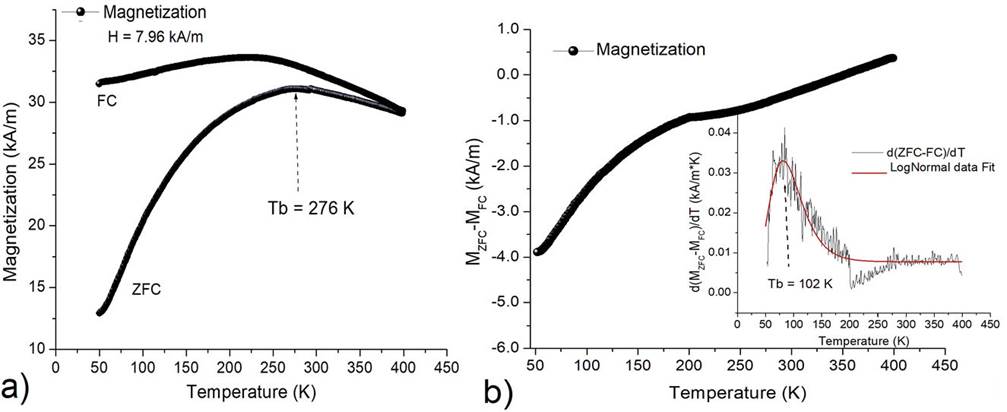
Figure 3 a) The dependence M vs T following the ZFC-FC protocol using H = 7.96 kA/m; b) the dependence (MZFC - MFC) vs T with the derivative in the inset, plus its corresponding LogNormal fit.
Then, the following experimental parameters are explicitly used in Eq. (1) to carry out the MC computer simulations: μ = μCS, T = 300 K, Vi = VCS, κ = 0; κ102; κ276, and the interval -2387 < H < 2387 kA/m. At the beginning of the simulation, the anisotropy axis of each particle

Figure 4 Dependences M vs H considering: a) κ = 0, κ102 and κ276; with randomly oriented, plus the experimental plot obtained via VSM; b) κ = 0, κ 102; with oriented in the directions
The dependence of the magnetization on the temperature is discussed now. The temperature interval in the VSM experiment was 50 < T < K, whereas in the MC simulation, it is not limited. In Fig. 5a), the curves for weak magnetic intensities, namely, H = 0, 0.796, 3.18 (with κ = 0, κ = κ102) and 7.96 kA/m are shown. As the acceptance rate of the MC simulation is drastically decreased below 20 K, we have restricted the analysis to the interval 20 < T < 400 K. In all curves, the magnetizations reached maximum values between 30 K and 40 K and suffers a significant decrease at 20 K. Above 100 K, all curves (except H = 0 kA/m) satisfy the Curie law, as can be observed in the corresponding plots 1/Χ vs T of Fig. 5b); all points almost collapse in a straight line. When κ = 0, it is found the lower slope (< 45%) because the magnetic susceptibility Χ has reached the highest value, showing a good agreement with the magnetization curve of Figs. 4a) and b). When the amplitude of H is very weak, the main contribution to the energy of the MHS is provided by the dipolar interactions Udd and the anisotropy energy Uanis. Further analysis of the rate Udd/Uanis exhibits Udd/Uanis ≈ 2/3 above 100 K and below Udd/Uanis ≈ 3/2. This last behavior agrees with the observations of the dipolar interactions in the FC trace of the magnetization obtained in Ref.21.
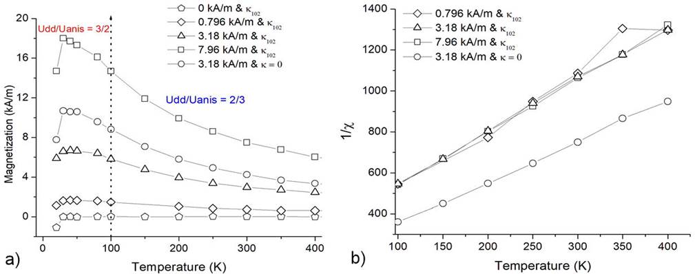
Figure 5 a) The dependences M vs T obtained via MC with different magnetic field intensities, κ = κ102, and κ = 0 plotted in the interval 20 < T < 400 K. b) The dependence 1/Χ vs T in the interval 100 < T < 400 K.
To highlight the importance of the dipolar interactions at low temperatures, in Fig. 6 configurations of the MHS (magnetized with H = 7.96 kA/m) are shown for two different temperatures, namely, 100 K and 20 K. The spheres are placed in the corresponding spatial positions and the arrows describe the orientation of the magnetic moments. As can be observed in the XYZ view and the XY projection, the orientations at 100 K have some random distribution. The opposite behavior is observed at 20 K, where the magnetic moments are aligned perpendicularly to

Figure 6 Thermalized configurations of the MHS inside of the simulation box in isometric views XYZ and the respective XY projections applying H = 7.96 kA/m
A discussion about the theoretical models for M applied to the experimental (MVSM) and the simulated curve (Mκ102) when

Figure 7 Magnetization MVSM superimposed with the corresponding Langevin equation (Eq. (3)), including MH (inset I) and ML (inset II).
Figure 8 shows the same qualitative analysis on M κ102 as in Fig. 7. In the full scale of H, the Langevin model again differs only near the transition to magnetic saturation. Nevertheless, inset (I) of Fig. 8 shows MH with a better agreement with MVSM. Moreover, in the inset (II) of Fig. 8, ML remains under the Langevin limit, even when the simulation has taken into account the dipolar interactions. This reinforces the idea that the initial slop of the experimental curve provided in the inset of Fig. 7 must be due to the presence of a fraction of particles where the anisotropy axis is aligned with the external field.

Figure 8 Magnetization Mκ102 superimposed with the corresponding Langevin equation (Eq. (3)), including MH (inset I) and ML (inset II).
5. Conclusions
A detailed characterization of a magnetite-dopamine core-shell nanoparticle sample was presented, including direct measurement of particle size through TEM microscopy, the thickness of coating using TGA, the blocking temperature and M vs H response, by vibrating sample magnetometry. Using those measurements, the parameters needed to carry out MC computer simulations were obtained. The dependence of H on the magnetization was studied by Monte Carlo computer simulations, using two possible magnetic anisotropy constants and three different orientations of the anisotropy axis
Last, but not least, we should point out that this work also provided a condensed derivation of the magnetization including different physical contributions, which might be implemented in further works to properly analyze the magnetization beyond the ideal Langevin equation.

