


 nova página do texto(beta)
 Inglês (pdf)
 Artigo em XML
 Referências do artigo
 Enviar este artigo por email
 Citado por SciELO
  Similares em
SciELO
Similares em
SciELO 
 Permalink
Without a doubt, one of the most important problems facing science today is that of explaining the accelerating expansion of the universe. Since 1998, with observations of SNIa-type supernovae it was established that the universe is experiencing a clear accelerated expansion contrary to the belief that the expansion must be slowing down due to the gravitational force of all matter in the universe itself. Since that time several independent tests have been conducted for the same observation, today there is no doubt that the universe is accelerating. The question has provoked an enormous amount of hypotheses and explanations, from the simple cosmological constant, proposed by Einstein himself to the modification of Einstein’s equations, massive gravity, hollographic universe, etc.
One of the beliefs is that the explanation for the acceleration of the universe could come from quantum mechanics, that is, from a theory of quantum gravity. This possibility is robust and has been explored by various scientific groups around the world, sadly without success. In the Ref. [1] they proceeded in an alternative way, because up to now we do not have a theory of quantum gravity, in this reference the authors propose an effective way to introduce the quantum character of the graviton, using analogies with other fields and interactions. They show that with this proposal the system behaves very similar to the ΛCDM case. The similarity was excellent and this hypothesis led to further studies. In this work we will show that the predictions of the ΛCDM and CMaDE models are indistinguishable, at least at cosmological scales, since the CMB and MPS profiles, the two strongest observations we have in the universe, are exactly the same, but the CMaDE model using an explanation of quantum mechanics without dark energy.
In this work we want to study a possible solution given in Ref. [1] for the last problem using very simple arguments for the gravitational interaction. The main goal of this work is not to convince the reader of the arguments given in Ref. [1] to find a form for dark energy, but to use this form as an effective function, a proposal to fit all the observations without free constants. In what follows we remain the main ideas of [1], but then we use the functional form of the dark energy in effective way.
The main arguments of [1] is that in the case of a massless particle, such as the gravitational interaction mediator or graviton, the energy due to its momentum E = pc, is not contained in the Einstein equations. In the Einstein’s equations it is implicit that the mass of the mediator of the gravitational interaction is zero. On the other side, the energy of the graviton due to its moment comes from the quantum mechanical character of the graviton. But everything in nature gravitates. The claim of [1] is that this energy also gravitates and must be counted as extra energy.
The hypotheses in Ref. [1] are: if Gravitation is a quantum mechanical interaction its mediator has a Compton effective mass and its corresponding wavelength λ is limited by the size of the observable universe. Using these arguments, they found that the cosmological constant is given by
We will use Λ as indicated in Ref. [1] as an effective result, where Λ varies very slowly, as we shall see.
For an observer today, the gravitational interaction travels a distance RH during its life, the wavelength will be λ = (c=H 0 )R H long, where R H is the unitless length
given in terms of the e-folding parameter N = ln(α=α0) and the Hubble parameter H = N , being a the scale factor of the universe and α0 its value today.
In order to obtain the Friedmann equation for our model, we consider that
here ρ m represents the matter density, ρ r corresponds to radiation density, k is the curvature parameter and ρ Λ = Λc2/k 2 is the dark energy density, where ·k = 8πG/c4 is the Einstein constant. Using Eqs. (1) and (2) in the derivative of (3), we get that [1]
where, for any given variable q, the prime means
From the above we have that the CMaDE Friedmann equation is given by (4).
Here it is important to note that given (1) with (2) for the function Λ implies that the
CMaDE model only has curvature as a free constant to fit all observations. If we
integrate (4) and (2) we find that
We obtain that
When inflation ends, the wavelength grows up about e
60 times thus
So far, the arguments used in Ref. [1] could be controversial for some readers; the objective of this work is not to discuss these arguments, but to see Eq. (1) with the integral (2) as an effective proposal and check if they can explain the observable universe, leaving for future work the possible quantum gravity explanation of the Eqs. (1) and (2) [2]. Note that this λ is similar to the proposal of holographic dark energy where we know that this model is not able to explain the dark energy behavior of the universe [3]. The difference of (2) with the holographic model proposal is that the holographic wavelength is the distance to the horizon of the universe, this integral has an extra scale factor outside the corresponding integral (2). The other main difference is that the holographic model has a free constant in the cosmological function Λ, while the Eq. (1) has no free parameters. So, let us think of the Eq. (1) as an effective proposal and its justification are the results that we find in this work.
Figure 1 we compare the numerical solution of (4)
with the evolution of the Hubble parameter in ΛCDM,

Figure 1 In the upper panel we show the evolution of the Hubble parameter using
the CMaDE ((4), point line) and the ΛCDM model (solid line). We used the
Planck values
Solving Eq. (4) numerically for a flat space-time we carry out the integral (2) and we find that R H =3.083 in Eq. (1). With these results we obtain that
where we can see that the value of ΩΛ strongly depends on the size of the wavelength (2).
We can use the size of the universe horizon to determine the value of the wavelength λ. Thus we can determine the value of the CMaDE now and give an explanation of the cosmological and coincidence problems.
In what follows we want to study the possibility that the CMaDE model is capable of
reproducing all the observations of the universe that we have so far. Strictly speaking
we have to solve (4) and solve the whole cosmology using it [1, 6]. However, in this work
we first solve the entire cosmology using an approximation. Here we will focus on the
temperature fluctuations of the cosmic microwave background (CMB) and the mass power
spectrum (MPS) only, leaving a more in-depth analysis of the rest for future work.
[6]. In order to find a suitable approximation
to the (4), we proceed as follows. We know that during the epoch dominated by matter
So, we find that the field equation for Λ
MD
is
However, this approximation is not good enough for the numerical solution of (4). Instead of that we will approximate it with the function
where q and Ω0Λ are constants that fit the numerical solution. The similarity between the function (10) with the numerical integration of (4) is very good everywhere, see Fig. 2.
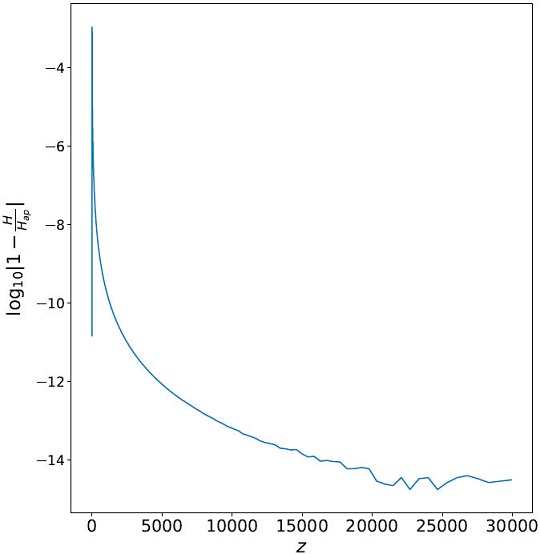
Figure 2 Evolution of the 1-H/H αpp using the numerical integration of (4) (H) and (10) (H αp ), with q=0.695. We plot log(|1-H/H αpp |), observe that this ratio is always less than 10-3.
The radiation content of the universe, CMB photons plus neutrinos, is given by
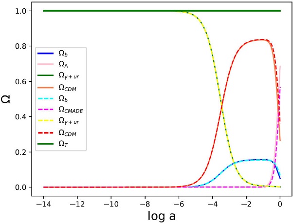
In Fig. 3 we see the evolution of the Ω’s for the CMaDE model, using the function (10) and the ΛCDM model, where we can observe the similarity of the evolution.
Thus, the next step is to see whether this approximation gives us the correct behavior of the CMB and MPS profiles. In Fig. 4 we show the comparison between the profiles of the CMaDE and ΛCDM models using an amended version of CLASS code [4], where, again, the similarity between both models is notable. The only difference we find for the flat universe is an excess of temperature predicted by the CMaDE model in the first maximum, but in the rest, of the two profiles, the coincidence with the observations using the Planck data is very good. It is remarkable that the value of ΩΛ in the CMaDE model is completely theoretical, so it is quite relevant that this match with the observations is so good. We believe that the small differences could be due to the fact that we are using an approximation for the CMaDE model and not the solution of the Eq. (4) or by some extra phenomenon. However, in this work we want to present the main characteristics of the CMaDE model, the observational aspects of the model will be found elsewhere [6].
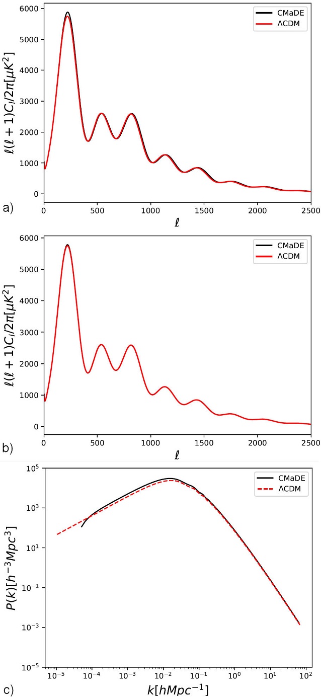
Figure 4 Profiles of the CMB for a flat universe (upper panel) and for a closed universe with Ω0k=-0.003 (middle panel) and MPS (lower panel) observations using an amended version of CLASS code [4]. We compare them with the best fit of the ΛCDM model, using data from the Planck satellite. Note that the CMB temperature fluctuations for the flat universe are the same as the ΛCDM, the only difference is in the first maximum. For the MPS there are very small discrepancies for the small structure. The CMaDE model settings are Ω0r=5.67×10⁻⁵, q=0.694, H 0 =72.6 km/s/Mpc and Ω0b=0.044 for the flat universe and q=0.695, Ω0k=-0.003, H 0 =72.6 km/s/Mpc and Ω0b=0.043 for the closed universe. Observe that the value of H 0 is very close to the observed one from the local distance ladder [5].
Finally, considering the gravitational field quantum nature we found that if it has a quantum Compton effective mass we could see it as a variable “cosmological constant". With this result, we could explain the actual value of the density parameter of the dark energy and the coincidence problem. Nevertheless, we think that this hypothesis opens a new window of research and must be further studied.

