


 nueva página del texto (beta)
 Inglés (pdf)
 Artículo en XML
 Referencias del artículo
 Enviar artículo por email
 Citado por SciELO
  Similares en
SciELO
Similares en
SciELO 
 Permalink
1. Introduction
The growing demand for energy sources to sustain the lifestyle of today’s societies has brought consequences to the environment, as well as public health problems in industrialized cities [1]. The use of fossil fuels as the main source of energy, leads to the generation of greenhouse gases, where more than 77% of the total concentration of anthropogenic gases corresponds to CO2 [2]. Despite the efforts and results achieved by the so-called renewable energies, oil and coal continue to be the principal energy sources, more than 60% of the energy produced comes from these two sources [3]. Different approaches have been proposed and evaluated to mitigate the effects of CO2, from capture and storage, to its reuse and conversion to high-value chemicals [4]. The reuse of CO2 for fuel production can be achieved through electrochemistry, traditional catalysts, and biological conversions [5-8]. However, these processes require considerable energy consumption, and result in high operating costs [9,10]. The transformation of solar energy into chemical bonds provides long-term energy storage [11, 12], whereas the photoreduction of CO2 to hydrocarbons is one of the breakthroughs in the field of photocatalysis. The materials used in the process of photocatalysis are responsible for absorbing sunlight, this absorption can create electron-hole pairs, that can migrate to the surface where they can be used for H2O dissociation and CO2 reduction [13-17]. The most common CO2 transformation leads to a product such as methane, methanol, formaldehyde, acid formic, etc., always demanding a high amount of energy since these are endergonic and non-spontaneous chemical reactions [18]. Although there have been multiple studies regarding the synthesis of efficient and stable photocatalyst [19, 20], only a few studies focus their attention on reaction engineering, as well as obtaining the optimal conditions for the reaction and the photoreactors design [21-26].
Two reactor configurations are used extensively for applications in CO2 reduction with photocatalytic methods, the continuous flow system and the batch system. The batch system is one of the most reported, however, its photocatalytic efficiency is low, becoming imprecise when compared to other methods [27]. The key limitation of the batch reactor system is the accumulation of products inside the reactor chamber for a defined time, which can lead to changes in the concentration of the reactants and reabsorption at the surface of the photocatalyst. Although continuous-flow reactors have better efficiency, the production of compounds is inadequate due to the short residence time of the reactants inside the reactor chamber, reducing the contact time with the photocatalytic material [28,29]. In this sense, the optimization of the residence time for continuous flow reactors, becomes a difficult problem to solve, as well the study of the fluid dynamics and the mass transfer, due to the geometric dependence presented by the fluid dynamics inside the reactor.
The optimization problem by deterministic methods for systems whose analytical representation cannot be solved traditionally, numerical methods and stochastic algorithms become a great alternative. One of the most popular stochastic methods, which belongs to the family of evolutionary algorithms, is the Genetic Algorithm (GA) [30]. This concept was first formalized by Holland [31], and later extended by De Jong for functional optimization [32]. GA uses search strategies inspired by the Darwinian notion of natural selection and evolution. During an optimization by GA, a set of solutions are chosen randomly, this set generates an offspring with the best characteristics of the previous population. This generation of offspring and selection is used recursively to get an optimum solution [33].
On other hand, Computational Fluid Dynamics (CFD) is a well-established tool for numerous areas of science and engineering [34-36]. CFD uses numerical methods and empirical approximations to solve the Navier-Stokes equations, and due to the development of numerical methods and advances in computational technology, there exists a growing confidence in the results of these computational methods. From the reactor design point of view, in the case of gas-solid reactors, the geometric complexity restricts detailed modeling of their fluid dynamics and, therefore, their optimization. In this sense, tools such as CFD, bring a trustworthy tool for solving fluid dynamics in gas-solid reactor systems [37-41].
In the present work, GA are used to maximize the residence time of the reactant phase inside a multi-inlet vortex photoreactor. CDF is used to solve the fluid dynamics inside each individual in the population of GA. The objective function as well as the statistics of residence time is reported and compared to the classic geometric configuration of multi-inlet vortex reactors. An analysis of turbulent intensities inside the photoreactor was implemented to determine the best operational conditions.
2. Methology
2.1. Optimization Process of the Prototype Reactor
2.1.1. Genetic Algorithm
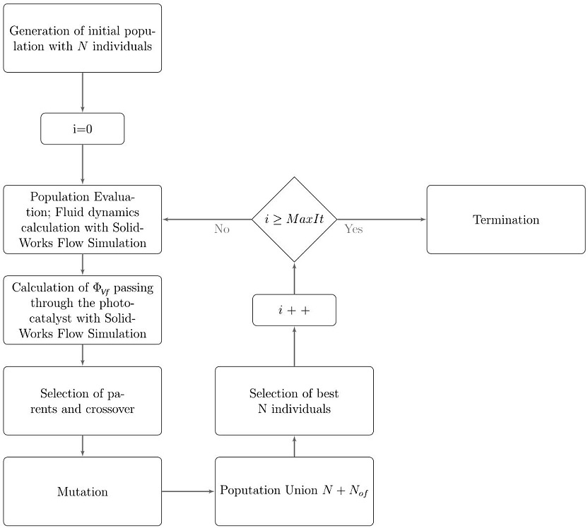
The importance of using the Genetic Algorithm in the present work lies in the wide range of possibilities to build a reactor device. Logically, there is a large number of configurations to arrange and set the reactant inlet, the product outlet as well as the catalyst support within the reactor vessel. This set of parameters must be evaluated which makes the process time and computer demanding. To initialize the reactor configuration selection, are required design values currently established, and afterward the algorithm randomly generates and evaluates the best generation of results, which are fit according to the objective function.
The implemented GA consists of six main steps, four of them correspond to the evolutionary loop, where the selection of parents, crossing, mutations, creation of offspring and the selection of individuals for the next generation takes place; the other two steps correspond to the initialization and termination of the evolutionary loop. The algorithm can find a local minimum of a real and real-valued objective function
1. Initialization. In this step, the first population (t 0) is generated with N numbers of individuals, each individual has a specific gene which is a vector with n design variables, chosen randomly values within their domain, each individual is evaluated with the objective function. Equation (1) shows the gene of the mth individual. In all generations there are N individuals.
2. Selection of parents and crossover. In this step, the individuals of the t i generation, with the best solution that minimizes the objective function are selected to perform crossover. The type of selection used corresponds to roulette selection, where the most outstanding individuals have a higher probability of being selected than the less outstanding individuals. Each individual evaluation by the objective function has a result, namely cost (c), a probability p m is assigned to each individual y m according to its c m , using Eq. (2).
where β is the selection pressure and
must be satisfied. Two individuals, namely parents v 1 and v 2, are chosen randomly accordingly to its probability p m , to perform crossover,
Each crossover creates two offspring, u 1 and u 2,
accordingly, to Eqs. (9) and (10).
in which
with
The selection of parents and the creation of offspring are executed until the number of offspring required N of is achieved.
3. Mutation. In this step, each offspring has a probability of changing some of the values of their gene, within a certain allowed range for each design variable, this process creates a changed version of the offspring, Eq. (13). Some design variables of the gene of the offspring are chosen randomly to change its value accordingly to Eq. (14).
where δ it is a number selected by a normal probability distribution with mean µ = 0 and selectable variance σ2.
4. Union of population and offspring. In this step, the current population (t i ) is joined with the offspring generated in the selection of parents and crossover step, giving a population size of N + N of .
5. Evaluation and selection. In this step, the N of offspring population is evaluated with the objective function, and the population N + N of is ordered accordingly to the individuals c m to select the best N individuals, these individuals generate the population of the generation ti+1.
6. Termination. In this step, it is determined whether it is necessary to end the evolutionary loop or to return to the Selection of parents and crossover step. The termination is done when the evolutionary loop reaches a maximum number of iteration (MaxIt), this is t MaxIt .
The GA parameters used in this work correspond to, MaxIt= 50; N = 10; N of = N; β = 1; γ = 0.25 and σ = 0.4. An in-house software based on Phyton, from the Python Software Foundation [45] (with headquarters in Delaware, USA), was developed to execute the GA.
2.1.2. Design Variables and Boundary Conditions
The proposed multi-inlet photoreactor, namely GA photoreactor, consists of three main components. First, a quartz window is located in the upper part that allows the passage of light. Second, a photocatalytic bed is placed in the lower part of the main chamber before the reactor outlet (the photocatalytic bed, for the CFD is isotropic with a porosity of 50% and a width of 1 mm). And, third, the reactor body where the main chamber is surrounded by the reactant gas inlets. Figure 1 shows the detail of the different parts of the photoreactor.

FIGURE 1 Multi-inlet vortex photoreactor components for Genetic Algorithm optimization: a) Exploded view of the multi-inlet vortex photoreactor components; b) Assembly of the multi-inlet vortex photoreactor components.
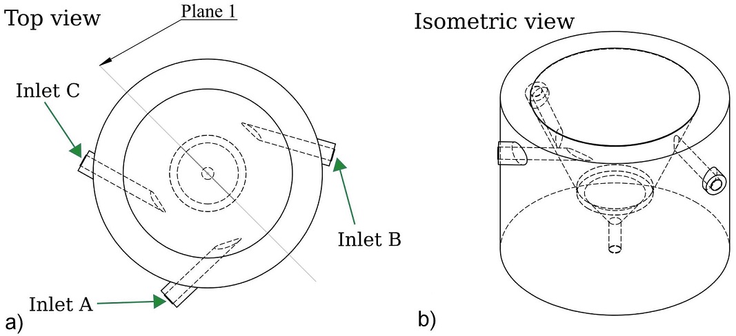
The geometric design variables, that modify the current GA photoreactor, add up to seven, refer to Fig. 2. Three design variables correspond to the angle around the main chamber of the three inlets, namely θ A , θ B , and θ C . These inlets are always tangent to the circle formed by the cut of the cone at their specific height, and have a diameter of 1.59 mm. Another three design variables are the height of the inlets, namely H A , H B and H C , all the heights are measured from the surface of the photocatalytic bed. Finally, the angle of the wall in the main chamber, which is labeled as θ D .

FIGURE 2 Design variables for the Genetic Algorithm: a) Shows the three design variables related to the height H of the reactant inlets as well as the design variable that controls the angled wall of the main chamber θ D ; b) Shows those design variables related to reactants inlets angle (θ A , θ B , and θ C ) around the main chamber.
Only two dimensions are kept constant, the height of the main chamber, with a value of 14.30 mm, and the diameter of the photocatalytic bed, with a value of 10 mm. The gene of the mth individual in the GA will be,
The maximum and minimum values for the design variables are shown in Table I. The limit values for θ A , θ B , and θ C were selected to ensure no superposition of the inlets.
TABLE I Limit values for the reactor design variables.
| Name | Maximum Value | Minimum Value |
| θ A | 360.0◦ | 310.0◦ |
| θ B | 168.0◦ | 70.0◦ |
| θ C | 288.0◦ | 190.0◦ |
| θ D | 150.0◦ | 90.0◦ |
| H A | 13.5 mm | 2.0 mm |
| H B | 13.5 mm | 2.0 mm |
| H C | 13.5 mm | 2.0 mm |
The objective function corresponds to the volume rate (Φ V f ml/min) that passes through the photocatalytic bed. In all the runs for the GA the three inlets have a volume flow rate of 83.3 ml/min with CO2 at 298 K, and the outlet has a pressure opening at 100 kPa, as boundary conditions for the CFD. A Flow chart for the implemented GA is shown in Fig. 3.
2.1.3. Computational Fluid Dynamics
All CFD software includes a representation of the NavierStokes equations, turbulence models and models that represent physical phenomena. In this work, the CFD software that was selected corresponds to SolidWorks Flow Simulation from Dassault Systèmes, with headquarters in Velizy-Villacoublay, France. This tool uses a modified k − ε twoequation turbulence model designed to simulate accurately a wide range of turbulence scenarios, and a boundary Cartesian meshing technique that allows accurate flow field resolution with low cell mesh densities.
Depending on the tested fluid and its conditions, any fluid flow can be classified as one of the following [46]:
Laminar. That is, a smooth flow without any disturbances.
Turbulent. This is a flow regime characterized by random vorticity and Eddie currents.
Transitional. An alternation between laminar and turbulent regions.
The modified k−ε turbulence model with damping functions proposed by Lam and Bremhorts, and used in SolidWorks Flow Simulation, describes laminar, turbulent and transitional flows of homogeneous fluids. This model employs two transport equations, one for the turbulent kinetic energy (k), Eq. (16), and the second for the turbulent dissipation (ε), Eq. (17) [47].
with
in which, C μ=0.09, C ε1=1.44, C ε2=1.92, σ ε = 1.30, σ B = 0.90, C B = 1.00 if P B > 0 and C B = 0.00 if P B < 0.
The turbulent viscosity is determined by:
The Lam and Bremhorst’s damping function f µ is determined by:
where,
In this case, y is the distance from a point to the wall and Lam and Bremhorst’s damping functions f 1 and f 2 are determined by:
The heat flux is defined by:
where, σ c = 0.9, Pr is the Prandtl Number, and h is the thermal enthalpy.
Another important quantity for analysis is the turbulence intensity, which is defined as,
where u 0 is the root-mean-square of the turbulent velocity fluctuations and U is the mean velocity (Reynolds averaged), and can be computed as
the mean velocity can be obtained from the three mean velocity components as
For each reactor design a global mesh of level 4, with an advanced channel refinement provided by SolidWorks Flow Simulation, was used for the determination of the fluid dynamics. The solver was configured to reach a steady-state.
For comparative purposes, a reference photoreactor was studied. The geometrical consideration for this reference photoreactor was of those from the classical configuration for multi-inlet vortex reactors [48,49]. In this reference reactor, gas feed inlets are at equidistant position each other and their heights are at the middle of the main cylinder, see Fig. 4. The criteria to evaluate the performance of both the optimized configuration of the prototype photoreactor and the reference, are the value of the turbulence and the residence time average. Because of this, a plane that cuts transversally both reactors is used, namely plane 1, this plane is depicted in Figs. 4 and 5 for optimized and reference photoreactor respectively.
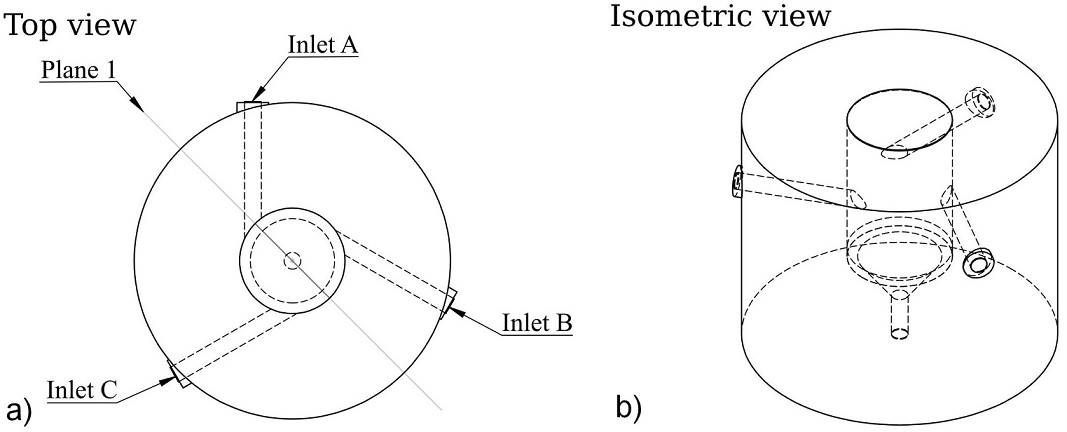
FIGURE 4 Reference reactor inlets configuration: a) Inlets and plane 1 for the cut plot. b) Isometric view of the reference photoreactor.
3. Results and discussion
3.1. Genetic algorithm
Throughout the optimization process, 500 reactor designs were simulated, and for each iteration of the evolutionary loop, the value of the best reactor desing Φ V f was obtained and plotted (Fig. 6). For the first five iterations there is a sharp decrease of Φ V f , suggesting a good performance of the GA. After iteration number ten, it can be seen that there is a slight change of Φ V f , indicating a local minimum approximation in the design space. After iteration number thirty there is no change in the Φ V f value, and the algorithm reaches a local minimum. The final values of the design variables are shown in Table II.

FIGURE 6 Calculated volumetric flow rate passing through photocatalytic bed after several iterations for the optimization process using GA.
TABLE II The optimized set of parameters for the reactor configuration, taken as indicated in Fig. 2.
| Name | Value |
| θ A | 313.4◦ |
| θ B | 74.0◦ |
| θ C | 240.9◦ |
| θ D | 113.0◦ |
| H A | 11.0 mm |
| H B | 7.20 mm |
| H C | 6.30 mm |
3.2. Residence time distribution and turbulence intensity
In order to find the residence time distribution for the optimized photoreactor (Opt) and the reference photoreactor a particle study was performed, where 30,000 representative particles of CO2 fluid were injected at each inlet, with a volume flow rate of 83.3 ml/min for all the three inlets. Figure 7 shows the residence time distribution for both photoreactors, it can be noted that the Opt photoreactor has a more uniform distribution with particles that stays longer in the reactor than the reference photoreactor. Also, the reference photoreactor has two main regions of time, the first between 0.1 s and 0.2 s, and the second, between 0.3 s and 0.6 s, whereas for the Opt photoreactor the main time region is between 0.5 s and 1.1 s. The mean residence time for the Opt photoreactor corresponds to 0.79 s, and for the reference photoreactor 0.29 s, this is an improvement of 2.7 times with respect of the reference photoreactor. This proves that with Φ V f as the objective function for the GA implementation, it is possible to adjust indirectly the residence time for this type of photoreactors.

Figure 8 shows the flow trajectories for the reference photoreactor and the Opt photoreactor. It can be seen from Figs. 8a) and 8b) that the higher part of the Opt photoreactor has more fluid lines than the reference photoreactor, this is an indication of better reactants distributions inside the Opt photoreactor. Figures 8c) and 8d) show the vortex formed in both photoreactors. It can be noted that the fluid trajectories for the reference reactor are concentrated near the cylinder wall, whereas for the Opt photoreactor its fluid trajectories are more concentrated at the middle of the cone wall. Moreover, it can be seen from this figure that molecules have to travel longer path in the Opt photoreactor, this has consequently that residence time becomes longer because of these larger trajectories within this optimized photoreactor.
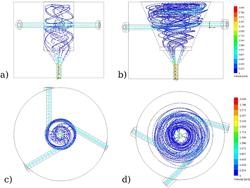
FIGURE 8 Flow trajectories: a) Reference photoreactor front view; b) Opt-3-Tuned photoreactor front view; c) Reference photoreactor top view; d) Opt-3-Tuned photoreactor top view.
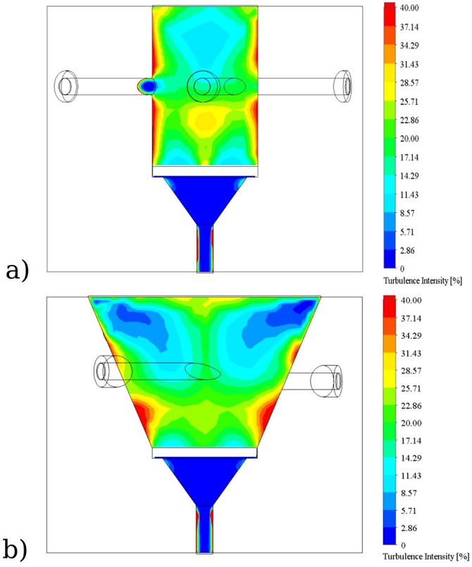
A cut plot on plane 1, showed in Figs. 9a) and b), was performed to find the turbulence intensities behavior inside both photoreactors. It can be observed that there are marked turbulent zones (more than 10%) near the photocatalytic bed in both cases. The case of the reference photoreactor reaches 14.5% turbulence intensity on the photocatalytic bed surface, whereas for the Opt photoreactor the average turbulence intensity onto the photocatalytic bed yields 15.5%. This turbulence intensity of the Opt photoreactor together with the high turbulence intensity near the photocatalytic bed ensures the mixing and contact of the reactant phases.
4. Conclusions
Computational Fluid Dynamics showed goodness in process operation and optimization in order to gain insight into the performance of a current designed and tailored photoreactor configuration. According to the simulation results, by changing the inlet angles and height, as well as the wall angle of the main chamber in the photoreactor, a higher residence time and turbulence are enhanced that, logically, in a multiphase system such as our planned reaction system, is essential for the reaction to occur. With the current study, reactor design and optimization lead to construct the physical device to perform the experimental study with the conviction that its performance will be optimal and the kinetic measurements will be intrinsic. The latter is the target of our further work and research.

