


 nueva página del texto (beta)
 Inglés (pdf)
 Artículo en XML
 Referencias del artículo
 Enviar artículo por email
 Citado por SciELO
  Similares en
SciELO
Similares en
SciELO 
 Permalink
1 Introduction
The transport of intensity equation (TIE) widely used in optics, is an equation that relates an optical wavefront W and the corresponding intensity distribution I at some detection plane after the output of some optical system to be tested [1,2]. In some works, this equation has been developed proposing that, under specific conditions it can lead to a Poisson equation [3,4]. The recovery of the optical wavefront is thereby reduced to a numerical problem [5], offering the advantage that the spatial resolution of the test will depend on the number of pixels of the detector and not only on the number of elements (stripes, lines, points) obtained by conventional tests that use spatial filters or complex optics like interferometric tests, Ronchi or Hartmann tests [6].
On the other hand, a general method has been developed to calculate the intensity of light that propagates in a medium whose refractive index n(r) varies slowly with the position, based on a differential equation of the curvature of the wavefronts [7]. In addition, there is a ray counting method for determining the PSF of an optical system by counting the rays that hits a hypothetical grid [8]. With these ideas in mind, we have developed an algorithm for calculating the intensity distribution from an optical wavefront using the ray counting method [9,10].The theoretical support of this algorithm is based on the ray propagation theory: for an isotropic and non-conducting medium, geometric rays are defined to be the orthogonal paths to the wavefront W(x, y); rays direction matches with the direction of the average Poynting vector [11,12]. In a perpendicular plane, relative to the propagation of the wavefront, the spatial distribution of the intensity due to the divergence and convergence of the rays along the observation plane can be obtained. The number of rays is the main parameter that leads to obtaining an approximate function of the luminous intensity at the detection plane. In this work, we obtain an approximation of the the characteristic intensity patterns of some aberrations, based on the calculation of the density of rays.
2 Zernike polynomials
Zernike polynomials are often used to express data from the wavefront in polynomial form, since they are constituted by terms whose graphs resemble the typical aberrations that we can observe in optical testing [13]. In polar coordinates, these polynomials are expressed as follows:
where the radial polynomials
In Cartesian coordinates the following transformations are considered [14]:
As an example, Table I shows the first six Zernike polynomials.
Table I First six orthogonal Zernike Polynomials.
| n | m |
|
Cartesian, Coordinates |
Polar Coordinates |
Name |
|---|---|---|---|---|---|
| 0 | 0 |
|
1 | 1 | Piston |
| 1 | 1 |
|
x | ρ sin φ | y-Tilt |
| 1 | 1 |
|
y | ρ sin φ | x-Tilt |
| 2 | 2 |
|
2xy | Ρ2 sin 2φ | Primary Astigmatism Axis at 45o |
| 2 | 0 |
|
-l + 2x2 +2y 2 | 2ρ 2-1 | Defocusing |
| 2 | 2 |
|
y2 - x2 | ρ2 cos 2φ | Primary Astigamtism Axis at 0o or 90o |
3 Transport of Intensity Equation
It has been shown in previous works that if a wavefront, which propagates in the direction of the optical axis, is considered within the paraxial approximation, we obtain the equation [6]:
where
If the intensity distribution is considered to be almost uniform, the first term of Eq. (4) vanishes and the TIE becomes a Poisson equation as follows:
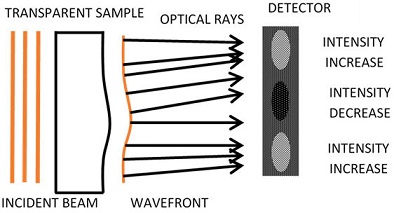
Although Eq. (5) may seems simple, in practice the analytical solution is too complex to carry out, so it is used to be solved numerically, taking the wavefront W as an unknown function, and the numerical values of the intensity calculated in two unfocused planes in the propagation axis as data input (Fig. 1), which is used to find the approximation to the derivative intensity corresponding to the term on the right-side of Eq. (5)

This derivative is known as the sensor function S and can be approximated as
Despite the considerable amount of work aimed at solving the TIE and obtain the wavefront, as far as we know, the inverse problem about obtaining function intensity from wavefronts has not been previously discussed.
To be more specific, some typical aberrations of optical surfaces can be recognized by patterns characterized by Ronchi patterns, patterns of Hartmann test, and interferometric techniques. However, there is no idea what the intensity pattern would looks like for optical testing techniques that use the TIE as a theoretical basis.
4 Ray counting method
As already mentioned, some authors have derived the TIE based on the Poynting’s theorem [11,12]. The main idea of these works is to calculate the density flow I of a surface element perpendicular to the direction of the vector intensity flux. Also, we assume an aberrated wavefront W coming from an optical system that is immersed in a homogeneous medium, which hits hits the surface of some flat detector. As the rays represent the direction of flow of radiant energy and they are perpendicular to the wavefront, there will be more iluminated areas than others on the detector surface due to the convergence or divergence of the optical rays, see Fig 2.
With this in mint an algorithm has been developed using the trace method and ray counting in order to find an approximate intensity function, using as input data a wavefront function which must fulfill the conditions where the TIE is valid (smooth surface or on the paraxial zone) [9].
Figure 3 shows a schematic of our ray counting algorithm. First, we assume that the value of any point of the wavefront Wi is known at the position xi. Next, we find the position

this equation gives us the direction of the rays.
Once the exact positions where the rays hit on the hypothetical detector are known, the algorithm must find these positions to their nearest integer index value from a mesh, such that all adjacent rays coincide in that position, as shown in Fig. 4.

For a given wavefront, this algorithm gives us the intensity distribution that must be compared with the actual intensity function.
5 Simulations
To obtain the characteristic intensity patterns of some aberrations, we propose the following algorithm
Select a Zernike polynomial (input function), corresponding to some aberration, like one of those presented in Table I, and obtain the numerical values of its function.
Calculate the intensity distribution functions at three different planes to calculate the sensor function S, as described in Eq. (6).
Apply a phase retrieve algorithm that uses the TIE to obtain an output function, as described in Sec. 4.
Finally, compare the rms wavefront differences and correlation values between the input and the output wavefront functions.
According with step 4, we consider that if these comparisons show us a similarity between the input and output wavefront functions, then the calculated intensity corresponds to that obtained using TIE techniques which it is the aim of this work.
6 Results
As example, we select the Zernike polynomial corresponding to astigmatism at

Now, with the trace and counting ray algorithms, we compute the intensity in three different planes (Δz = 0.02 mm) to calculate the sensor function according to Eq. (6). In Fig. 6 we observe the results of these calculations, which are similar due to the plane nearest where they are placed.
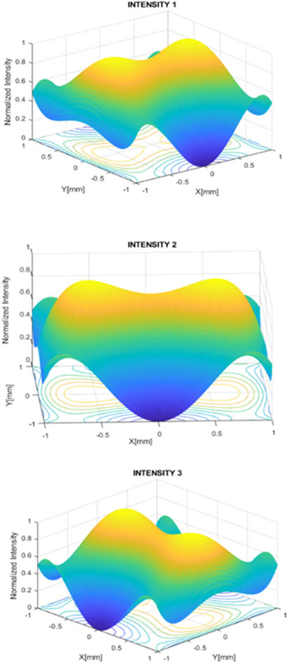
Figure 6 Intensity patterns calculated with the counting and tracing method ray, for astigmatism aberration.
Then, the Poisson numerical solution algorithm was used in rectangular coordinates to retrieve the wavefront. The retrieve output wavefront is show in Fig. 7. A qualitative comparison between the input (Fig. 5) and the retrieved wavefront (Fig. 7) shows the similarity of both plots.

Next, for quantitative comparison, we calculated the difference between the input and retrieved output wavefront. The error differences are shown in Fig. 8. Here, the rms error differences and correlation values for astigmatism at 90o error function are 12.11 × 10⁻⁴ and 0.9932, respectively.

Additionally, to evaluate the performance of our proposed method other higher-order Zernike polynomials were evaluated. The results of our simulations are shown in the plots of Fig. 9. Here, the analyzed wavefront aberrations were a) Primary astigmatism axis at 45o, b) Triangular Astigmatism 30o, 150o, 270o, c) Coma along x-axes, d) Coma along y-axis, e) Triangular Astigmatism 0o, 120o, 240o, f) Ashtray 22.5o, g) Fifth-order Astigmatism axis at 45o, h) Spherical Aberration, i) Fifth-order Astigmatism axis at 0o or 90o, and j) Ashtray 0o, respectively. From a qualitative point of view, the graphs recovered with our method resemble the original input aberrations.

Figure 9 Higher order wavefronts evaluated with the proposal method. a) Primary astigmatism axis at 45o, b) Triangular Astigmatism 30o, 150o, 270o, c) Coma along x-axes, d) Coma along y-axis, e) Triangular Astigmatism 0o, 120o, 240o, f) Ashtray 22.5o, g) Fifth-order Astigmatism axis at 45o, h) Spherical Aberration, i) Fifth-order Astigmatism axis at 0o or 90o, j) Ashtray 0o.
On the other hand, the correlation and rms values between the original and the retrieved wavefront are shown in Table II. We can observe that almost all the aberration functions can be retrieved with accuracy, with rms differences ranging from 9.93 × 10⁻⁴ to 22.99 × 10⁻⁴. However, for some aberration functions there are small correlation values, for example, for fifth-order Astigmatism axis at 0o or 90o. In this case, the corresponding retrieved plot (Fig. 9i)) does not resemble completed the original aberration function. We think that this issue could be solved if we increase the number of rays used in the simulation.
Table II Correlation and RMS values between original wavefront and those recovery with ray-tracing algorithm.
|
|
Name | Correlation (C) | RMS × 10-4 |
|---|---|---|---|
|
|
Primary Astigmatism axis at 45o | 0.9791 | 14.96 |
|
|
Primary Astigamtism Axis at 0° or 90° | 0.9932 | 12.11 |
|
|
Triangular Atigmatism 30°, 150°, 270° | 0.9648 | 18.22 |
|
|
Coma along x axes | 0.7004 | 22.99 |
|
|
Coma along y axes | 0.7004 | 22.99 |
|
|
Triangular Atigmatism 0°, l20°, 240° | 0.9648 | 18.22 |
|
|
Ashtray 22.5 | 0.9955 | 19.59 |
|
|
Fifth-order Astigmatism, axis at 45° | 0.8581 | 12.21 |
|
|
Spherical Aberration | 0.89045 | 9.93 |
|
|
Fifth-order Astigmatism, axis at 0° or 90° | 0.5768 | 17.50 |
|
|
Ashtray 0 | 0.9518 | 21.57 |
7 Conclusions
The method proposed here was developed and tested with different Zernike aberration polynomials. The calculations of the rms wavefront differences and correlation values between the original and retrieved wavefront show an accurate relationship that validates the method. The retrieve wavefront can be recovery with an accuracy that ranges between 9.93 × 10⁻⁴ to 22.99 × 10⁻⁴ for some wavefront aberrations. In addition, it was found that this method helps us to validate all the algorithms developed. We conclude that our proposed method is useful to identify aberrations in optical testing workshops when phase retrieve techniques supported by the TIE are used.

