SciELO - Scientific Electronic Library Online

 
vol.67 número6Analysis and electronic circuit implementation of an integer and fractional-order Shimizu-Morioka systemNonlinear dynamical properties of solitary wave solutions for Zakharov-Kuznetsov equation in a multicomponent plasma índice de autoresíndice de materiabúsqueda de artículos
Home Pagelista alfabética de revistas  

Servicios Personalizados

Revista

Articulo

Indicadores

Links relacionados

  • No hay artículos similaresSimilares en SciELO

Compartir


Revista mexicana de física

versión impresa ISSN 0035-001X

Rev. mex. fis. vol.67 no.6 México nov./dic. 2021  Epub 14-Mar-2022

https://doi.org/10.31349/revmexfis.67.061502 

Research

Plasma Physics

An eigenvalue analysis of damping in optical thin plasmas

J. Fajardoa  c 

P. Contrerasb  c 

M. H. Ibañez S.c 

aFacultad de Ciencias Básicas, Educación, Artes y Humanidades, ITSA, Barranquilla, Colombia.

bDepto de Física, Universidad de Los Andes, Mérida 5101, Venezuela.

cCentro de Física Fundamental, Universidad de Los Andes, Mérida5101, Venezuela.


Abstract

In this work, the behavior of magnetohydrodynamic waves in optically thin plasmas considering dissipative processes, thermal and magnetic diffusion, a given ionization, and the heating and cooling functions are investigated for several particular cases. A numerical eigenvalues analysis of the dimensionless secular equations according to various cases is performed for the entire set of MHD equations.

Keywords: Thin optical plasmas; magnetosonic waves; Alfvèn waves; thermal waves; magnetic diffusion; astrophysical plasmas

PACS: 52.35.Bj; 52.30.Cv; 52.35.Mw; 52.25.Dg; 52.25.Xz

1.Introduction

In recent years analytical as well as numerical tools for working out nonlinear partial differential equation and, in particular, those governing general fluids have been enormously improved. Nonetheless the linear problem resulting from analyzing these equations remains to be very important for many reasons:

  • The associated eigenvalue problem describes the behavior of magnetohydrodynamic waves (MHD) and other waves, for example, thermal and radiation waves.

  • Understanding the behavior of linear waves allows to understand many physical aspects of nonlinear problems like the onset of the turbulence as well as its closed relation with it 1-5.

  • The linear approach is closely related to the problem of stability of different flows and gas structures in different physical fields such as in astrophysical problems: planetary atmospheres, Earth’s oceans, stellar interiors 3,6,7 stellar atmospheres (e.g., the solar atmosphere), interstellar medium, and intracluster media 8,9.

However, the present work is limited to the analysis of some aspects of MHD wave propagation in optically thin plasmas of interest in astrophysics. Extensive efforts have been put into practice for the solar atmosphere 10-24 and the interstellar and intracluster media 14,25-27.

We consider several aspects in the Alfvèn wave damping analysis and in the magnetosonic wave analysis and the associated eigenvalue problem for optically thin plasmas, as will be seen and discussed at the present work.

In Sec. 2, the set of MHD equations is linearized, leading to two independent cases where each matrix generates a dispersion relation whose roots for the case of Alfvèn waves are a complex equation.

In Sec. 3, for the linear approximation both modes are studied for the thermal and magneto-acoustic cases. They are damped by thermal conduction, viscosity and the influence of the cooling-heating function. The complex eigen-equation is both described in the case where only one dissipative process is considered and where only the magnetic diffusion term ν̃m is present.

In. Sec. 4, the energy equation is used without any dissipative terms but preserving the effects of the heat/loss given its importance in astrophysical and laboratory plasma applications.

Finally, in Sec.5, the kinetic coefficients in a magnetic field, for the case of a recombining hydrogen plasma are discussed.

2.General set of magnetohydrodynamic equations

If dissipative effects are accounted for a recombining gas, for an optically thin and heat conducting plasma, the well known basic MHD equations can be written as 16,20,25,28

Hkxk=0, (1)

Hit=-ϵijkxjvjHk-vkHj+c24πσ2Hixk2, (2)

ρt+(ρvi)xi=0, (3)

dξdt+X(ρ,T,ξ)=0, (4)

ρdvidt=-pxi+14πxk(HiHk-12H2δik)+σ´ikxk, (5)

ρTdsdt=-ρL(ρ,T,ξ)+xiκikTxk+c216π2σ[-ϵjkiHjxk]2+σikvixk, (6)

and

p=N0kBμ(ξ)ρT, (7)

where Hi and v i are the i-th components of the magnetic field and velocity, respectively. ϵjki is the permutation symbol 𝛿 𝑖𝑘 is Kronecker delta symbol, the light speed and ρ, p, T, ξ, c v , N0, kB and μ(ξ) are mass density, pressure, temperature, ionization degree, specific heat at constant volume, the Avogadro number, the Boltzmann constant and the mean molecular weight of the gas, respectively.

X(ρ,T,ξ) is the net ionization rate and L(ρ,T,ξ) is the heat-loss function defined as energy losses minus energy gains per unit mass and time, which can be written as L(ρ,T,ξ)= L(ρ,T,ξ)output-L(ρ,T,ξ)input.

Additionally, κik and σik are the thermal conduction and the viscous stress tensor, respectively.

The thermal conduction coefficient κik is generally weakly dependent on density but strongly dependent on temperature 19,29-31.

Strictly speaking the induction equation becomes rather complicated, in particular, the electrical conductivity σ is also a tensor, however, for sake of simplicity and taking into account that σ/σ=1.96, this quantity will be assumed as a scalar of magnitude 𝜎 and the induction equation will be assumed in the simplified form given by Eq. (2) 30.

This set of equations reduces to the known MHD equations when the heat/loss term is neglected.

3.Eigenvalue analysis of the type of magneto hydrodynamic waves

For an inert plasma, if all dissipative processes are neglected, Eqs.(1), (3) and (7) hold and Eqs.(2)-(6) simplify, i.e the set of ideal MHD equations can be written as

H=0, (8)

Ht=×(v×H), (9)

ρt+(ρv)=0, (10)

dvdt=-1ρp-14πρH×curl(H), (11)

st+vs=0. (12)

For small disturbances superposed to an steady flow with velocity V 0, magnetic field H 0, pressure p0 and mass density ρ0 16,32

v=V0+v',H=H0+h,p=p0+p',ρ=ρ0+ρ',

where v´, h´, p´ and ρ' are functions of (x,y,z,t). Therefore, Eqs.(9)-(12), up to the first order, become

h=0, (13)

ht-×(v'×H0)-×(V0×h)=0, (14)

p't+V0p'+ρ0u02v'=0, (15)

v't+(V0)v'+1ρ0p'+14πρ0H0×curl(h), (16)

where ρ'=p'/u02+(ρ/s)ps' and u02=(p/ρ)s is the square of the adiabatic sound speed, and

s't+V0s'=0. (17)

By Fourier analysis one can write the space and time dependence of the perturbed variables as exp[ikr-ωt]. Equatios (13)-(16) reduce to

kh=0, (18)

-ωh-k×(v'×H0)-k×(V0×h)=0, (19)

V0k-ωp'+ρ0u02kv'=0, (20)

V0k-ωv'+1ρ0p'k+14πρ0H0×(k×h) =0, (21)

and

V0k-ωs'=0. (22)

Equation (18) implies that h is perpendicular to k, therefore, from Eq.(21) if p´= 0, Eqs.(20) and (22) reduce to

V0k-ω=0,s'0,k×v'0. (23)

Without loss of generality, V 0 and H 0are assumed to be on the x - y plane. The above relations define an entropy vortex wave which is carried along with the flow and is independent of other linear modes which correspond to the solutions

V0k-ω0,s'=0,kv'=0. (24)

These modes are defined by the eigenequations

u-VxHxHx4πρuhzvz=0, (25)

and

(u-Vy-HyHxHx4πρ0u-Hy4πρ(u-Vx)-u02u-Vx0)(hyvxvy)=0, (26)

where u=ω/k is the phase velocity. Herein after, the subindex zero indicating equilibrium values will be omitted, except for the adiabatic sound speed u0. k is taken here to be along the x-axis.

In the particular case of a plasma initially at rest, the compatibility conditions for the Eqs. (25) and (26) become

u2=Hx24πρ, (27)

and

u4-H24πρ+u02u2+Hx24πρu02=0. (28)

As it is well known, Eqs.(25) and (27) define the Alfvèn modes, and Eqs.(26) and (28) define the fast and slow magnetosonic modes (Alfvèn suggested the existence of hydro-magnetic waves in 1942) 16,32.

In the general case of a plasma flowing with an initial constant velocity V 0 the dispersion relations are modified accordingly but the nature of the wave modes remains.

In conclusion, as far as the linear approximation concerns, there are three kind of waves in a plasma flow, and which are independent each other:

  • The entropy-vortex modes.

  • The Alfvèn modes.

  • The magnetosonic waves.

The entropy entropy-vortex modes were worked out in 31,33.

4.Dissipative processes in magneto hydrodynamic waves with a given ionization and heat/loss effects

For a plasma with a given ionization and taking into account dissipative and heat/loss effects, the linearization of Eqs.(1)-(7) give, as in the ideal case, two sets of equations independent from each other, that is

ω+ic2k24πσHxkHxk4πρω+iηk2ρhzvz=0, (29)

where c is the light velocity, σ is the conductivity coefficient, and η is the kinematic viscosity.

ω(-iω+Ω)0iu02ρω+Γk00ω+ic2k24πσ-kHykHx-k-Hyk4πρω+i4η3+ζk200Hxk4π0ρω+iηk2p'hyvxvy=0, (30)

where γ is the ratio of specific heats c p /c v , κ is the thermal conductivity, ζ is the bulk (second) viscosity, and Ω and Γ are given by

Ω=1cvκk2ρ+LT,Γ=ρ(γ-1)[ρLρ-T(κk2ρ+LT)], (31)

with the derivatives of the heat-loss function Lρ=L/ρ, and LT=L/T.

We should notice that the coefficients of viscosity appearing into the viscous stress tensor, are tensors due to the anisotropy introduced by the magnetic field, in this case the ratio between the parallel and perpendicular kinematic viscosity becomes η/η1.98, therefore, the kinematic viscosity as well as the bulk viscosity can be assumed as scalars of magnitude η and ζ, respectively, in Eqs.(29) and (30).

Additionally, the strong anisotropy inherent in the thermal conduction tensor ( κijη/η10-12) has been taken into account assuming the heat flux vector to be

q=-κTsn+κTsn, (32)

where n and n are unit vectors along and perpendicular to H 0, respectively.

Therefore,

κ=κcos2θ+κsin2θ, (33)

where θ=cos-1Hx/H0.

In dimensionless form Eq.(30) can be written as

1+i(κ̃k̃2+L̃T)0-1+iγ-1(L̃ρ-L̃T-κ̃k̃2)k̃001+iν̃mk̃2-sin(θ)k̃cos(θ)k̃-β2k̃-sin(θ)k̃1+i43ν̃+ν̃bk̃200cos(θ)k̃01+iν̃k̃2p̃'h̃yṽxṽy=0 (34)

where

κ̃=κωρcva2cos2(θ)+κκsin2(θ), (35)

and k̃=ak/ω,a=H0/4πρ, L̃T=LT/cvω, L̃ρ=ρLρ/cvTω, ν̃=ωη/ρa2, ν̃b=ωζ/ρa2, ν̃m=ωc2/4πσa2, β=u0/a, p̃=p/ρu02, h̃y=hy/H0, ṽx=vx/a, and ṽy=vy/a.

4.1.Numerical results for the Alfvèn wave damping

The corresponding dimensionless secular equation of the system of equations (29) becomes equal to

ν̃ν̃mk̃4+1-iν̃+ν̃mk̃2-1=0, (36)

where ν̃=ωη/ρax2, ν̃m=ωc2/4πσax2, k̃=axk/ω and ax=Hx/4πρ.

The roots of Eq (36) are complex, that is, k̃=k̃r+ik̃i where k̃r and k̃i are real quantities.

Due to the fact that ν̃ as well as ν̃m ( l¯/λ1, where l¯ is the mean free path and λ the Alfvèn wave length , the quartic term of Eq.(36) can be neglected and the resulting quadratic equation has the solution sought.

k̃i12ν̃+ν̃m. (37)

Because the disturbance has been taken in the form exp(kr-iωt), therefore ki=ωk̃i/ax becomes the absorption coefficient.

One must remark that the expression 37 holds as far as the damping per wave length is very small. This expression is obtained by in a different way.

Strictly speaking if both coefficients ν̃ and ν̃m are different from zero, Eq.(36) has two roots for k̃2, however only one of the roots fulfils the condition k̃i1 for which the present approximation holds.

For this physical meaningful mode, the velocities (v), the damping coefficient (k i ) the damping per unit wave length (ld/λ=kr/2πki) and the ratio hz/vzπρ have been plotted in 1 as functions of ν̃ for three different values of of the ratio v m /v(=0.1 blue line, 1 black line and 10 red line).

Additionally, for the (k i ), the damping per unit wave length, the Landau approximation for (37) has been plotted (3 pointed lines in Fig. 1b)).

Figure 1 The velocity modes (v) a), the damping coefficient (k i ) b), the damping per unit wave length (l d = λ = k r =2πk i ) c), and the ratio hz/vzπρ d) have been plotted in Fig. 1 as functions of 𝑣 for three different values of of the ratio v m /v (= 0:1 blue line, 1 black line and 10 red line) 

4.2.Numerical results for the magnetosonic and thermal waves

The condition of compatibility of the system of Eqs.(34) can be written as

(a0r+ia0i)k~8+(a1r+ia1i)k~6+(a2r+ia2i)k~4+(a3r+ia3i)k~2+1+iL~T=0, (38)

the coefficients αkl are defined as

a0r=κ~ν~ν~m(43ν~+ν~b),a0i=β2γ-1κ~ν~ν~m,a1r=β2γ-1κ~(ν~+ν~m)+κ~[ν~1+13cos2θ+ν~bcos2θ]+ν~ν~m[β2+43ν~+ν~bL~T],a1i=β2γ-1[κ~cos2θ+ν~ν~mL~T-L~ρ]-κ~[ν~(43ν~+ν~b+73ν~m)+ν~bν~m]-ν~(43ν~+ν~b)ν~m,a2r=β2γ-1ν~+ν~mL~T-L~ρ-κ~73ν~+ν~b+ν~m+ν~1+13cos2θ+ν~bcos2θL~T-[ν~(43ν~+ν~b+73ν~m)+ν~bν~m]+β2cos2(θ),a2i=β2γ-1L~T-Lρcos2θ-κ~-κ~-ν~43ν~+ν~b+73ν~m+ν~mν~bL~T-[ν~(β2+1+13cos2(θ))+ν~bcos2(θ)+β2ν~m] ,a3r=-[(73ν~+ν~b+ν~m)L~T+1+β2],

and

a3i=β2γ-1L̃ρ-L̃T+κ̃-L̃T+73ν̃+ν̃b+ν̃m. (39)

Generally speaking, the parameters defining the coefficients of the fourth order polynomial in k̃2 (38) depend on two thermodynamic quantities, say, ρ and T and two quantities defining the magnetic field, i.e. H and θ. Therefore, these parameters define the corresponding four wave modes resulting from the Eq. (38).

The square root ±k̃ represents two waves propagating in opposite directions each other. The angle ranges between 0θ π/2, but the ranges for ρ, T and H where the dispersion relation (38) holds is rather wide.

Therefore, here only a few asymptotic cases will be discussed and the solution of the full polynomial (38) will serve only for specific applications.

If all dissipative mechanisms as well as the heat/input effects are neglected and θπ/2, the dispersion relation reduces to a quadratic polynomial for k̃2 (28) corresponding to the undamped fast and slow magnetosonic waves (mw) 16 but when θ = π/2 only the fast magnetosonic mode remains.

If the only dissipative process taken into account is the thermal conductivity and θπ/2, Eq.(38) reduces to a cubic polynomial the roots of which correspond to two damped magnetosonic waves sw and a thermal wave Thw.

When θ = 0 a root becomes k̃=1 for which p̃'=0 and ṽx=0, corresponding to an undamped Alfvèn wave 𝐴𝑤 with values of h̃y/ṽy=1.

The other two roots with
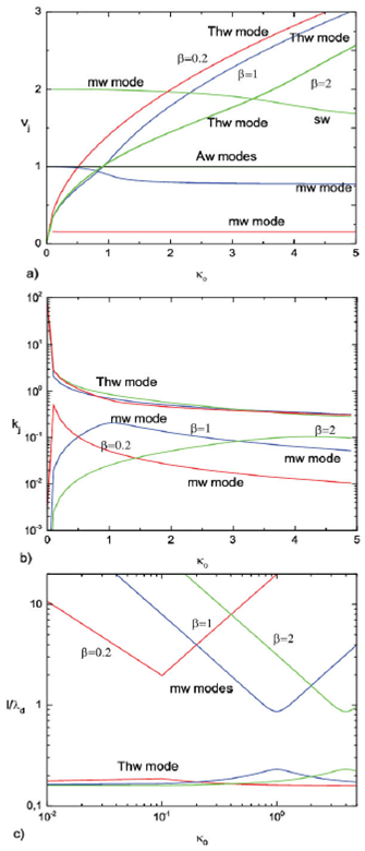
 k̃1 are a damped magnetosonic wave sw and an over damped thermal wave Thw for which p=ρωvx/k, all of which are plotted in Fig. 2.

Figure 2 For the θπ/2 case the phase velocity a) is plotted for three different values of β = 0:2 (red lines), 1 (blue lines), 2 (green lines) are shown in the case of a thermal mode Thw and the sw mode, also the undamped Alfvèn mode Aw is the solid black line for the three cases. The damping coefficient b) and the damping per unit wave length c) are plotted for three different values of β = 0:2 (red lines), 1 (blue lines), 2 (green lines). 

In Fig. 2, the phase velocity a), the damping coefficient b) and the damping per unit wave length c) are plotted for three different values of β = 0.2 (red lines), 1 (blue lines), 2 (green lines) as function of κ0.

Note that the maximum damping of the magnetosonic wave (red mw line, occurs at the same value of κ0 at which the maximum damping of the thermal wave occurs for the three β Thw values in Fig. 2b) 10,12.

If θ = π/2 the dispersion equation reduces to a quadratic equation, one root becomes a damped thermal wave and the another one a damped magnetosonic wave for which ṽy=0, |h̃y/ṽx|=|k̃|, and |p̃/ṽx|=β2|(1-k̃2)/k̃|, see Fig. 3 where the above two wave modes are plotted for = 0.2 (red lines), β = 1 (blue lines), β = 2 (green lines) for both mw and Thw modes.

Figure 3 For the dispersion Eq. (38) using the thermal conductivity with θπ/2, the two wave modes mw and Thw are plotted for β = 0:2 (red lines), β = 1 (blue lines), β = 2 (green lines). In this figure however, the wave parameters have been plotted as function of κ-=κω/ρcva2 instead of κ-||

Here one must emphasize that in the figures above the wave parameters have been plotted as function of κ̃=κω/ρcva2 instead of κ̃, i.e. the scales involved here are quite different (by a factor of the order of 1012) from those involved in Fig. 2.

For an angle θ0 and θπ/2 there are three modes, one thermal and two magnetosonic waves (the fast and slow) modes, for which the amplitudes are related by

|h~yv~y|=1|k~cos(θ)| ,|v~xv~y|=1|k~2[sin(θ)-cos(θ)]cos(θ)|,|p~´v~y|=|1+γ-1κ~k~31+κ~k~2||v~xv~y|, (40)

Figure 4 corresponds to an angle θ=π/4 and the same values of β, i.e. β = 0.2 (red lines), β = 1 (blue lines), β = 2 𝛽=2(green lines). It can be observed a small jump in the phase velocity Fig. 4a) for the case of β = 1, which is reflected also in the amplitude Fig.4d).

Figure 4 Solution for the dispersion Eq. (38) using the thermal conductivity with θπ/4. a) Here the phase velocity, b) the damping coefficient, c) the damping per unit wavelength and d) the amplitude p-/v-x, are plotted for the two slow and fast mw modes, and the thermal Thw mode with β = 0:2 (red lines), β = 1 (blue lines), and β = 2 (green lines), it can be observed a small jump in the phase velocity a) for the case of β = 1, which is reflected also in the amplitude d). 

For this particular value of θ=π/4, h̃y=ṽy=0, and |p̃/ṽx|=|(1+γ-1κ̃k̃3)/(1+κ̃k̃2)|.

The thermal waves show a minimum of p̃/ṽx at the value of κ̃0 at which the maximum damping per unit wave length ld/λ occurs.

The magnetosonic wave showing its minimum of ld/λ at lower value of κ̃0 presents an increasing value of p̃/ṽx when κ̃0 increases, but the magnetosonic wave with its minimum occurring at a larger value of κ̃0 has a decreasing ratio p̃/ṽx when κ̃0 increases.

If only the magnetic diffusion (ν̃m) is accounted for, there should be no thermal waves because only the magnetic terms are considered. In this case the dispersion Eq.(38) reduces to a quadratic equation for k̃2 for which |p̃/ṽx|=1. Furthermore, for θ = 0, a root becomes k̃=1/β2, i.e. an undamped mode for which hy = 0 and vy = 0 , and the other root becomes k̃=i/(i+ν̃m).

Figures 5 and 6 show the results for θ = π/4 and π/2 respectively, and three different values of β = 0.2 (red lines), β = 1 (blue lines), β = 2 (green lines). The the amplitude in these cases is p̃/ṽx=1.

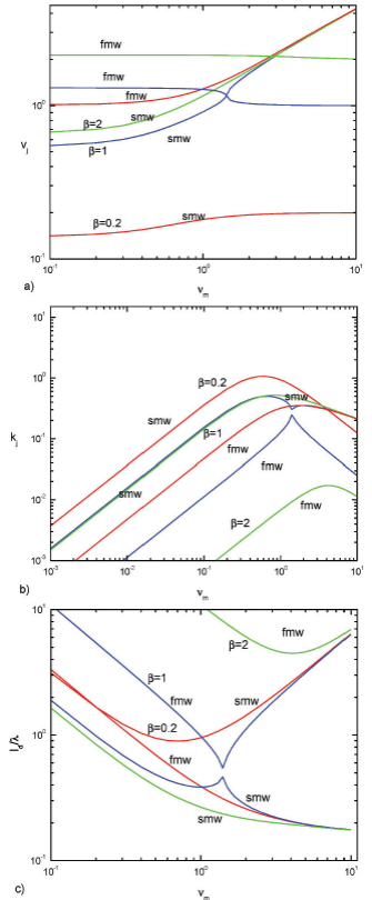
Figure 5 a) The phase velocity, b) the damping coefficient, and c) the damping per unit wavelength for the magnetosonic fast and slow modes are plotted for β = 0:2 (red lines), β = 1 (blue lines), β = 2 (green lines), for the dispersion Eq. (38) as function of the magnetic diffusivity with θπ/4, for β = 1 (blue line), a crossing of slow and fast magnetosonic modes is observed. 

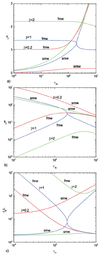
Figure 6 a) The phase velocity, b) the damping coefficient, and c) the damping per unit wavelength for the magnetosonic fast and slow modes are plotted for β = 0:2 (red lines), β = 1 (blue lines), β = 2 (green lines), for the dispersion Eq. (38) as function of the magnetic diffusivity with θπ/2, for β = 1 (blue line), a crossing of slow and fast magnetosonic modes is observed. 

When the magnetic energy density is of the order or larger than the kinetic energy in the wave β ≤ 1 , there is no crossing of slow and fast modes, but mode crossing occurs when β = 1, see Figs.5a) and 6a) for two examples.

The damping coefficient for the slow mode is a decreasing function of ν̃m (∼ω) but that for the fast mode shows a maximum at a value of ν̃m depending on the value of 𝛽 (Figs. 5b) and 6b)) and for the damping per wavelength there is a corresponding minimum (Figs. 5c) and 6c)). This minimum occurs at the mode crossing point when β = 1.

Furthermore, for θ=π/2, ṽy=0 and |h̃y/ṽx=|k̃/(1+iν̃mk̃2)|.

The case when only thermal conduction and heat/loss effects are accounted for in the equations, but neglecting the viscosities and the magnetic diffusion as well as the above asymptotic cases, but neglecting the anisotropy effects of the thermal conduction coefficient, have been analyzed in a previous work 12.

4.3.Numerical analysis of the effect of the heat/loss function in the magnetosonic modes

The case when in the energy equation the dissipative terms are neglected but the effects of the heat/loss are considered deserves further analysis, because this particular case is of great importance in many astrophysical as well as laboratory plasma.

In this case the Eq.(38) reduces to a quadratic equation in k̃2 (if θπ/2) corresponding to two magnetosonic waves modified by the heat loss input.

For θ = 0 one root becomes k̃=1 corresponding to an undamped Alfvèn wave for which |h̃y/ṽy|=1 and the other root corresponding to the magnetosonic wave becomes k̃=γ(i-L̃T)/[iγ-L̃T-L̃ρ].

For θ = π/2, this is the only one root, but in this case, the magnetosonic wave has ṽy=0.

As a first approximation, the heat/loss function can be parameterized by the form

L(ρ,T)=ρϕi(T)-C0ρa-1TTib, (41)

ϕi(T) being the piece-wise function ϕi(T)=ΛiT/Tiη, where Ti and η are parameters depending on the interval of temperature under consideration (see Table I, 22).

Additionally, the parameters C0, a and b depend on the heating processes considered. In particular:

  1. For a constant per unit volume heating a = 0 and b = 0.

  2. For a constant per unit mass heating heating a = 1 and b = 0.

  3. Heating by coronal current dissipation a = 1 and b = 1.

  4. Heating by Alfvèn mode/mode conversion a = b = 7/6.

  5. Heating by Alfvèn mode/anomalous conduction damping a = 1/2 and b = -a.

See for instance 18,22 and references therein.

From Eq.(41) it follows that

L̃ρ(ρ,T)=2-aη-bL̃T, (42)

L̃T(ρ,T)=η-bρΛiTicvωTTiη-1. (43)

The cooling function Φi has been plotted as a function of temperature in Fig. 7a) in magenta color.

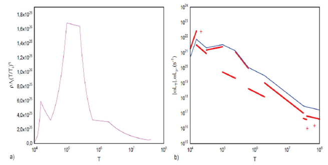
Figure 7 For gases with solar abundances (a completely ionized gas (ξ = 1) and a particle density n = pN0μ = 1) the cooling function Φi (T) has been plotted as a function of temperature in a) in magenta color, the derivatives ωL-T(ρ,T) (red thick line) and ωL-T(ρ,T) (blue thin line) as function of T have been plotted in b) for a constant heating per unit volume (case 1). 

The derivatives |ωL̃T(ρ,T)| (red thick line) and ωL̃ρ(ρ,T) (blue thin line) as function of T have been plotted in 7b) for a constant heating per unit volume (case 1), for a completely ionized gas (ξ = 1) and a particle density n = ρN0/μ= 1.

The intervals of temperature where L̃T(ρ,T)>0 are indicated with the red label +, elsewhere L̃T(ρ,T)<0.

The plots corresponding to the cases (2) to (5) also are shown: 8a) for a constant per unit mass heating, Fig. 8b) shows the heating by coronal current dissipation, Fig. 8c) plots the heating by Alfvèn mode/mode conversion, the heating by Alfvèn mode/anomalous conduction damping is shown in Fig. 8d).

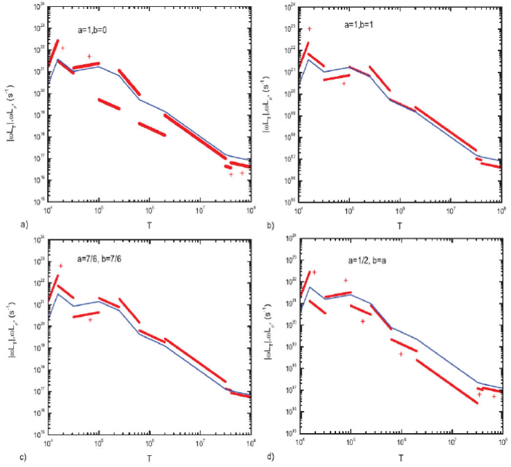
Figure 8 The heat/loss function derivatives ωL-T(ρ,T) (red thick line) and ωL-T(ρ,T) (blue thin line) as function of T, that correspond to cases (2) to (5) are shown in a) to d) for a completely ionized gas (ξ = 1) and a particle density n(pN0= μ) = 1. 

Due to the fact that the cooling term in Eq. (41) as well as its derivatives with respect to temperature and density are ∼ρ , for other densities, the corresponding values simply must be multiplied by the factor n.

5.Kinetic coefficients for a Hydrogen ionization plasma

At this Section the kinetic/dissipation coefficients in a magnetic field, for the case of a recombining hydrogen plasma will be quoted out and briefly discussed.

According 16,19,30,35,36, for a hydrogen gas with ionization 𝜉 the two electric conductivity tensors are respectively given by

σ=6.97×10⁷T3/2lnΛ, (44)

and

σ=1.96σ;

The thermal conduction coefficients are expressed as

κ=2.50×10³(1-ξ)T1/2+1.84×10-5ξT5/2lnΛ, (45)

and

κ=1.48×10⁻¹⁷ξ2n2H2T1/2, (46)

Finally, the kinematic viscosity coefficient is given by

η=2.21×10⁻¹⁵T5/2lnΛ, (47)

and the kinematic viscosity is expressed as

ν=ηρ. (48)

The logarithmic coefficients InΛ are for temperatures T < 4.2 x 10⁵ K

lnΛ=23.24+ln(10-4T)3nξ1/2

or when the temperature T < 4.2 x 10⁵K

lnΛ=29.71+ln10-6T(nξ)1/2.

On the other hand and as a first approximation, the total dissipative coefficient for magnetosonic waves can be written as

γd43ν+(γ-1)χ+νm, (49)

where χ = κ/ρcp is the thermometric conductivity and vm the magnetic diffusion 35-37.

Note that in the present approximation v(T), vm(T) , and χ(n,T, ξ) explicitly depend on the particular form of the rate function χ(n,T, ξ) and the wave frequency 25,37,38. In Ref. 38 the problem of reacting gases and the bulk viscosity has been discussed to some extent.

In Fig. 9a) the quantities 4v/3 (black solid line) and (γ-1) χ have been plotted as functions on temperature for n = 1 and four values of the ionization ξ = 10-6 (blue colour), 10-3 (red colour), 10-1 (brown colour), and 0.99 (green colour).

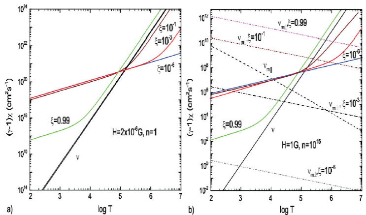
Figure 9 In a) (without magnetic diffusion) and b) (with (vm)), the quantities 4v/3 (black solid line) and (γ- 1)X have been plotted as functions on temperature for four values of the ionization ξ = 10 -6 (blue colour), 10-3 (red colour), 10 -1 (brown colour), and 0; 99 (green colour). 

Note that χ ∼ n2, therefore, the effect of increasing (decreasing) the density is to increase (decrease) the respective values of χ. The value of v m << 1010 cm-2s-2 in the range of T under consideration has not been plotted.

However, v m parallel and perpendicular to the magnetic field can become of the order or greater than of (4/3)v and (γ-1) χ for high densities (n ≥ 1010 cm-3) and strong magnetic fields H ≥ 1 G, for instance, in the solar low atmosphere and photosphere.

For context, in Fig.9b) all dissipation coefficients are shown for H = 1 G and n = 1015 cm-3; from where it is apparent that the magnetic dissipation parallel (v m ) as well as perpendicular (v m⊥ ) to the magnetic field becomes dominant in range of temperatures depending on the particular values of the ionization degree as well as the particle density.

In Fig. 9b) the quantities 4v/3 (black solid line) and (γ-1) χ have been plotted as functions on temperature for 𝑛=1 and four values of the ionization ξ = 10-6 (blue colour), 10-3(red colour), 10-1(brown colour), and 0.99 (green colour).

The perpendicular magnetic diffusion (v m⊥ ) is plotted is Fig. 9b) for four values of the ionization ξ = 10-6 (gray point line), 10 −3 (black point line), 10-1(brown point line), and 0.99 (magenta point line). The parallel magnetic diffusion (νm) is also plotted is 9b) (dash black line).

6.Conclusions

The present work was aimed at investigating the behavior and propagation of MHD waves in optically thin plasmas, with ionization and dissipative effects. The results are summarized in four sections.

In Sec.2, the set of MHD equations was linearized, leading to two independent cases where each matrix generates a dispersion relation whose roots for the case of Alfvèn waves are a complex equation.

In Sec. 3, for the linear approximation it was observed that both, thermal and magneto-acoustic modes are damped by the thermal conduction, viscosity and the influence of the cooling-heating function. The complex eigen-equation was described with some detail, and several asymptotic cases of the full polynomial solutions were discussed (38):

  • The case when the only dissipative process taken into account is the thermal conductivity was discussed for several values of θ in Eq. (38). We found eigenvalues corresponding to two damped magnetosonic waves, and a thermal wave. We also found a small jump in the phase velocity for magnetosonic modes for the case of β = 1 which is reflected also in the amplitude.

  • In the case with only the magnetic diffusion term (ν̃m), the dispersion Eq.(38) reduces to a quadratic equation for k̃2 for which |p̃/ṽx|=1 and lacks the thermal mode. It was found that if the magnetic energy density is of the order or larger than the kinetic energy in the wave for β = 1, a crossing of slow and fast magnetosonic modes was observed.

In Sec. 4, in the energy equation the dissipative terms were neglected, but the effects of the heat/loss were accounted, because of its great importance in many astrophysical as well as laboratory plasma applications. In this case the Eq. (38) reduces to a quadratic equation in k̃2 corresponding to two magnetosonic waves modified by the heat loss input. We described in this section five heating processes for a thin optical plasma.

Finally, in Sec. 5, the kinetic coefficients in a magnetic field, for the case of a recombining hydrogen plasma were briefly discussed. It was found that the magnetic dissipation parallel (v m ) as well as perpendicular (v m⊥ ) to the magnetic field become dominant in a range of temperatures depending on the particular values of the ionization degree ξ as well as the particle density n.

Acknowledgments

This work is dedicated to the memory of Prof. Miguel H. Ibañez S. (1945 - 2020) who devoted his life to the theoretical study of astrophysical plasmas and fluid dynamics in reacting gases, and non-adiabatic flows.

He always will be remembered as a devoted researcher, a teacher of several generations of Venezuelan physicists, and a unique friend.

We deeply thank an anonymous reviewer whose technical comments and language annotations helped improve and clarify this manuscript.

This research did not receive any grant from either the University of Los Andes or a government organization.

References

1. T. J. Dennis and B. D. G. Chandran, Turbulent Heating of Galaxy-Cluster Plasmas, Astrophys. J 622 (2005) 205, https://doi.org/10.1086/427424. [ Links ]

2. A. Burkert, The turbulent interstellar medium, C. R. Phys. 7 (2006) 433, https://doi.org/10.1016/j.crhy.2006.05.001. [ Links ]

3. P. Hennebelle and T. Passot, Influence of Alfvén waves on thermal instability in the interstellar medium, Astron. Astrophys. 448(2006) 1083, https://doi.org/10.1051/0004-6361:20053510. [ Links ]

4. L. Pan and P. Padoan, The temperature of interstellar clouds from turbulent heating, Astrophys. J. 692 (2009) 594, https://doi.org/10.1088/0004-637X/692/1/594. [ Links ]

5. H. Braun and W. Schmidt, A semi-analytic model of the turbulent multi-phase interstellar medium, Mon. Not. R. Astron. Soc. 421 (2012) 1838, https://doi.org/10.1111/j.1365-2966.2011.19889.x. [ Links ]

6. E. Parker, Cosmical magnetic fields: Their origin and their activity, (Clarendon Press, Oxford, 1979). [ Links ]

7. C. Heiles and T. H. Troland, The Millenium Arecibo 21 Centimeter Absorption-Line Survey IV: Statistics of Magnetic Field, Column Density, and Turbulence, Astrophys. J. 624 (2005) 773, https://doi.org/10.1086/428896. [ Links ]

8. W. H. Kegel and G. Traving, On the Jeans Instability in the Steady State Interstellar Gas, Astron. Astrophys. 50 (1976) 137. [ Links ]

9. R. Kippenhahn and A. Weigert, Stellar Structure and Evolution (Springer, Heidelberg, 1990). [ Links ]

10. M. H. Ibáñez S., Sound and thermal waves in a fluid with an arbitrary heatloss function, Astrophys. J. 290 (1985) 33, https://doi.org/10.1086/162957. [ Links ]

11. M. H. Ibáñez S. and N. M. Sánchez D., Propagation of Sound and Thermal Waves in a Plasma with Solar Abundances, Astrophys. J. 396 (1992) 717, https://doi.org/10.1086/171754. [ Links ]

12. M. H. Ibáñez S. and O. B. Escalona T., Propagation of Hydrodynamic Waves in Optically Thin Plasmas, Astrophys. J. 415(1993) 335, https://doi.org/10.1086/173167. [ Links ]

13. R. B. Dahlburg and J. T. Mariska, Influence of heating rate on the condensational instability, Sol. Phys. 117 (1988) 51, https://doi.org/10.1007/BF00148571. [ Links ]

14. G. B. Field, Thermal Instability, Astrophys. J. 142 (1965) 531, https://doi.org/10.1086/148317. [ Links ]

15. D. Giaretta, Polynomial Dispersion Relations, Astron. Astrophys. 75 (1979) 273. [ Links ]

16. L. D. Landau and E. M. Lifshitz, Electrodynamics of Continuous Media, 1sted. (Pergamon Press, Oxford, 1960). [ Links ]

17. D. Mihalas, Stellar Atmospheres, 2nd ed. (Freeman & Co., San Francisco, 1978). [ Links ]

18. R. Rosner, W. H. Tucker and G. S. Vaiana, Dynamics of the quiescent solar corona, Astrophys. J. 220 (1978) 643, https://doi.org/10.1086/155949. [ Links ]

19. L. Spitzer, Physics of Fully Ionized Gases (Interscience Publishers, New York, 1962). [ Links ]

20. T. H. Stix, Waves in Plasmas (Springer, Berlin, 1992). [ Links ]

21. J. T. Mariska, The Quiet Solar Transition Region, Annu. Rev. Astron. Astrophys. 24 (1986) 23, https://doi.org/10.1146/annurev.aa.24.090186.000323. [ Links ]

22. J. F. Vesecky, S. K. Antiochos, and J. H. Underwood, Numerical modeling of quasi-static coronal loops I: Uniform energy input, Astrophys. J. 233 (1979) 987, https://doi.org/10.1086/157462. [ Links ]

23. N. Kumar and P. Kumar, Viscous Damping of Non-Adiabatic MHD Waves in an Unbounded Solar Coronal Plasma, Sol. Phys. 236(2006) 137, https://doi.org/10.1007/s11207-006-0128-z. [ Links ]

24. B. Roberts, Waves and Oscillations in the Corona, Sol. Phys. 193 (2000) 139, https://doi.org/10.1023/A:1005237109398. [ Links ]

25. M. H. Ibáñez S., Damping of sound waves propagating in optically thin plasmas, Phys. Plasmas 11(2004) 5190, https: //doi.org/10.1063/1.1792633. [ Links ]

26. D. W. Goldsmith, Thermal Instabilities in Interstellar Gas Heated by Cosmic Rays, Astrophys. J. 161 (1970) 41, https://doi.org/10.1086/150511. [ Links ]

27. C. F. McKee and J. P. Ostriker, A theory of the interstellar medium: three components regulated by supernova explosions in an inhomogeneous substrate, Astrophys. J. 218 (1977) 148, https://doi.org/10.1086/155667. [ Links ]

28. J. Fajardo, M.Sc. thesis, 2016. [ Links ]

29. E. N. Parker, Instability of Thermal Fields, Astrophys. J. 117 (1953) 431, https://doi.org/10.1086/145707. [ Links ]

30. S. I. Braginskii, Transport Processes in a Plasma, in Reviews of Plasma Physics, edited by M. A. Leontovich (Consultants Bureau, New York, 1965), Vol. 1. [ Links ]

31. M. H. Ibáñez S., Entropy-vortex waves in non-adiabatic flows, Astrophys. J. 818 (2016) 119, https://doi.org/10.3847/0004-637X/818/2/119. [ Links ]

32. M. H. Ibáñez S., The stability of optically thin reacting plasmas: effects of the bulk viscosity, Astrophys. J. 695 (2009)479, https://doi.org/10.1088/0004-637X/695/1/479. [ Links ]

33. M. H. Ibáñez S. and L. A. Núñez, On the Vortex Waves in Nonadiabatic Flows, Astrophys. J. 855 (2018) 19, https://doi.org/10.3847/1538-4357/aaaa22. [ Links ]

34. M. H. Ibáñez S. and S. M. Conde, Heating of a Recombining Plasma by Bulk Viscosity Dissipation of Sound Waves, Rev. Mex. Astron. Astrofis. Ser. Conf. 40 (2011) 188. [ Links ]

35. L. D. Landau and E. M. Lifshitz, Fluid Mechanics, 2nded. (Pergamon Press, Oxford, 1987). [ Links ]

36. E. M. Lifshitz and L. P. Pitaevskii, Physical Kinetics (Pergamon Press, Oxford, 1981). [ Links ]

37. S. Conde, M. Sc. thesis, Universidad de Los Andes, 2010. [ Links ]

38. M. H. Ibáñez and P. L. Contreras, Damping of SoundWaves by Bulk Viscosity in Reacting Gases, Can. J. Pure Appl. Sci. 13 (2019) 4897. [ Links ]

Received: April 08, 2021; Accepted: May 12, 2021

Creative Commons License This is an open-access article distributed under the terms of the Creative Commons Attribution License