


 nueva página del texto (beta)
 Inglés (pdf)
 Artículo en XML
 Referencias del artículo
 Enviar artículo por email
 Citado por SciELO
  Similares en
SciELO
Similares en
SciELO 
 Permalink
1.Introduction
The history of the relation between Physics and Finance dates back at least to the pioneering work of L. Bachelier 1, published more than a century ago. However, it was not until recent decades that a growing and well-established body of research using tools from Physics, and particularly statistical mechanics, to understand economic phenomena through time series analysis had emerged 2,3. To cite just a few recent examples, in Refs. 4,5 the authors apply random matrix theory to study cross-correlations in financial markets in order to describe various market states and state transitions, while in Ref. 6, a microscopic model for automatically done high-frequency transactions is presented, using tools from the kinetic theory of gases. Our work is framed in this tradition, branded as Econophysics, from which the problem of the so-called market efficiency, here discussed, has by no way escaped.
It is important to establish that when speaking of the efficiency of the markets, two great perspectives of analysis must be distinguished: the so-called distributive efficiency and the informational efficiency. It is to the second approach to which we dedicate this work. The informational efficiency of prices is defined as the immediate incorporation of all relevant information for the formation of prices through the interaction in the markets of highly sophisticated economic agents.
Introduced by Fama in Ref. (7), it has important implications for the theory, in particular, that the differences of the logarithms of the consecutive prices of assets in a market must follow a (Gaussian) random walk. This hypothesis has been widely questioned, for example, in Ref 8,9.
One of the most common explanations for the inefficiency of real markets has been the “animal spirit” of Keynes 10, that is, the psychological and emotional factors that lead investors to make their decisions in capital markets when there is uncertainty, how human emotions can drive making financial decisions in uncertain and volatile environments.
Another explanation comes from the work of H. Simon 11, through the concept of limited rationality, that postulates that most people are only partially rational and act on emotional impulses without rational foundations in many of his actions.
Various authors, such as Lo in Ref. 12 and McCauley in Ref. 9 for example, recover the elementary fact that financial markets are, like all social phenomena, of a historical and dynamic nature, that is, agents respond to their specific social, political, psychological and technical conditions, which is why it is inappropriate to postulate general and anti-historical hypotheses about their behavior.
As indicated in Ref. 8, in recent years, most of the operations in the large financial markets have been automated and are now computers and not human beings who make decisions by executing certain algorithms. Although in the last decades, evidence has accumulated against the efficiency of the traditional markets, one could imagine that, with the execution of orders controlled by computer algorithms, devoid of feelings and emotional decisions, efficiency could be achieved in financial markets. Thus, the following question arises: are automated markets more or less efficient than classical ones? That is, what happens to efficiency if, in the process of incorporating the relevant information for price formation, human beings are replaced by algorithms?
The objective of this work is to offer evidence, through the analysis of time series of automated transactions in the US and Mexican markets, that the use of computational algorithms in automated high-frequency markets has not led these markets to the efficiency prescribed by the neoclassical theory. The organization of the paper is as follows: Section 2 develops the theoretical framework in which the analysis will be carried out. Section 3 describes the characteristics of the data and the methodology used for our analysis. In 4, the results obtained are discussed. Section 5 contains the conclusions. Section 6 contains the bibliography used.
2. Theoretical framework
The informational efficiency of a market implies that the consecutive price differences must be independent. Indeed, if there were any correlation between consecutive prices, it could be used to perform arbitrage, an action that would be in contradiction with the assumed efficiency. Thus, one can examine the short-term movement patterns that describe the returns of the assets in the market in question and attempt to identify the process underlying those returns. If the market is efficient, the model will not be able to identify a pattern, and we will conclude that the returns follow a random walk process. If a model is able to establish a pattern, past market data can be used to predict future market movements and the market is therefore inefficient.
Note that the observation of a random walk is a necessary condition for efficiency. There are studies that show that this condition is not sufficient 13,14. Consequently, the deviations of a random walk allow rejecting the informational efficiency of the assets under study.
The method that we will use has its origins in the work of Hurst 15, framed in the context of his
studies in hydrology and later refined by Mandelbrot and Wallis 16. Given a time series
x
n, x 𝑛 , n = 1,…,m with mean
Hurst noted that the rescaled range of the time series of annual flows of the Nilo
river as a function of the length n of the series was asymptotically a power law
when n tends to infinity:
In general, a Hurst exponent H greater than 0.5 is associated with the long-term persistence of the series: the range grows faster than expected from a random walk, that is, movements in one direction follow, with greater probability, movements in the same direction; while H < 0.5 is associated with long-term antipersistence: the range grows more slowly than that of a random walk, that is, movements in one direction are more likely to follow movements in the other direction, this on average and for large enough lengths. In both cases, the deviation of H from its hypothetical value 0.5 can be taken as a long-term memory measure: the movements of the series are not independent of the remote past.
The study of long-term correlations measured by Hurst exponent has been applied in Physics, for example, in 17 to the ion saturation current fluctuations and Ref. 18 to gamma, ray data. In the context of the financial time series that concerns us here, this long-term memory translates into deviations from market efficiency.
The remaining part of this section will be devoted to briefly discuss the approaches in the literature that will be used in the next section to define our methodology, as well as some results related to those of this work.
In Ref 19, it is argued that, given
a sequence of independent and identically distributed random variables, the shape of
the probability distributions of the random variables affects the Hurst exponent of
the series. The authors calculate the Hurst exponent Hstock for the daily
series of the S&P500 index. Then, they shuffle the series in order to remove its
memory, after which they calculate the Hurst index of the shuffled series, denoted
by Hperm (actually, this process of shuffling and calculating is repeated
a certain number of times, Hperm is defined as the mean and the standard
deviation is reported). The difference between Hstock and
Hperm is an indicator of the memory of the original series, while if
Hperm is different of 0.5. This is attributed to the distributions of
the variables, since the shuffled series are, by construction, memoryless. It is
proposed then to use Hperm as an indicator of lack of memory, instead of
the canonical value 0.5; that is,
In Ref 20, it is argued that the
R/S statistic is sensitive to short-term correlations so that if for a time series
is obtained
In Ref 22,23, the need to observe the evolution of the efficiency, measured by the Hurst exponent, over time is stated. The first article uses one-minute resolution data from 1983 to 2009 from the SP500. The Hurst exponent of the daily subseries is calculated, and a decreasing evolution is observed from 0.8 towards 0.5, with a statistically insignificant difference for the period 2005-2009. Similar results are obtained for the monthly exponents. For the purposes of this project, it is important to underline their explanation of the phenomenon: they attribute it to the growth of algorithmic trading. In the second article, daily exponent series are studied of eleven emerging markets between 1992 and 2002, with similar results.
Other perspectives on market efficiency by studying Hurst exponent had been proposed in the past. Very interesting is the discussion in Ref. 24, in which the authors study a measure of quantitative correlation between theoretical inefficiency and empirical predictability for 60 financial indices from different countries. The Hurst exponent is taken as a measure of market inefficiency, while to measure predictability, they use one of the most basic techniques of supervised machine learning: Nearest Neighbor (NN) and its proportion of correct answers. A considerable positive correlation (around 60%) between inefficiency and predictability is reported.
In Ref 25, it is shown that before the great economic collapses of 1929, 1987, and 1998 a clear decrease in the Hurst exponent from the persistence regime (H > 0.5) to the anti-persistence regime (H < 0.5) is observed.
In Ref 26, Peters carries out an extensive analysis of the R/S statistic, the relevance of which he argues through the Fractal Market Hypothesis (FMH) as an alternative to the Efficient Market Hypothesis (EMH). The fractal properties of the financial time series would be due to the differences in the time horizons of the financial agents, who, according to their interests, incorporate certain pieces of relevant information into the price of an asset that is not relevant for other time horizons. Market stability is attributed to the dynamic interaction of these different scales.
3.Nature of the data and methodology used
The data used in this investigation are the time series of prices of the automated (algorithmic) operations that occurred from March 7, 2018, to March 7, 2019, in the Mexican and US markets (251 trading days). For the US market, there were 539,834,024 records, and for the Mexican market, 78,863,574 records.
The importance for this work that our data comes from fully-automated transactions cannot be overstated: it is for this alone that we can test efficiency specifically for digital markets.
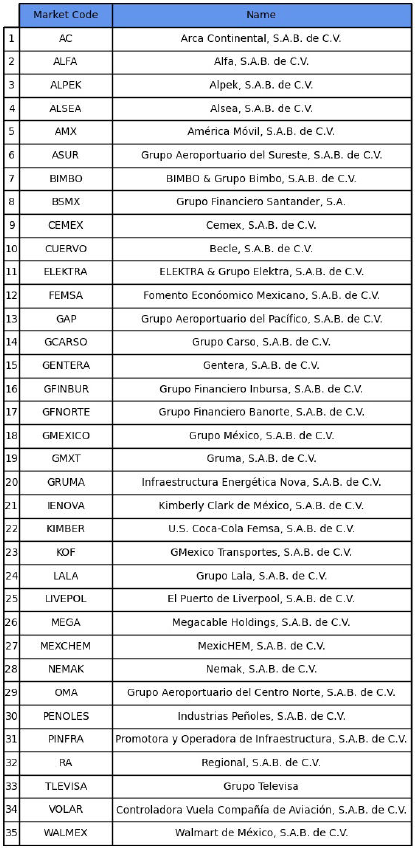
The data belongs to 59 assets; of these, 35 correspond to companies listed on the Mexican stock exchange: AC, ALSEA, ALPEK, ALPHA, AMX, ASUR, BIMBO, BSMX, CEMEX, CUERVO, ELEKTRA, FEMSA, GAP, GCARSO, GENTERA, GFINBUR, GFNORTE, GMEXICO, GMXT, GRUMA, IENOVA, KIMBER, KOF, LALA, LIVEPOL, MEGA, MEXCHEM, NEMAK, OMA, PENOLES, PINFRA, RA, TLEVISA, VOLAR, WALMEX; while the other 24 are from the US market: ABT, BAC, BMY, C, CSCO, F, FB, FOXA, GE, GM, HPQ, INTC, KO, MDLZ, MO, MS, MSFT, ORCL, PFE, TWTR, T, USB, WFC, VZ. The details can be seen in Fig. 1 and 2.

The following analysis is carried out for the series of logarithmic returns
where x(t,τ) is the t-th term of the series of means of τ seconds of logarithms of the prices of a given asset.
The Hurst exponent of a time series is obtained as follows: Given n less than the
length of the series, we calculate R/S of all subseries of length n of the original
series and define
To analyze the evolution of the Hurst exponent throughout the period under study, which is one year, we calculate the Hurst exponent Hstock of subseries of a certain number N of days, slid one day at a time 23. For example, if N = 5, the Hurst exponent of the first five days of the series is calculated, then that of the series that goes from the second to the sixth day, etc., and the last calculation is for the series of the last five days, with which the evolution of the weekly Hurst exponent Hstock throughout the year is obtained.
There is no satisfactory analytical theory for the R/S statistic; most of the results on the subject are derived from computer simulations, which implies that they depend on particular models. Thus, although R/S is non-parametric, it is usually used to test the null hypothesis of Gaussian random walk 26, so its rejection may be due to non-Gaussianity or short-term memory. That is why the methodology that will be used below to establish the statistical significance of our calculations, inspired by the proposals discussed in Secc .2, is based on global and local permutations of the series in question 19,21,23.
Continuing with the previous example with N = 5, for each subseries of five days of the original series, we shuffle its terms to destroy its memory, and the Hurst exponent is calculated for this new randomized subseries. The process of shuffling and calculating the Hurst exponent is repeated one hundred times, thus obtaining a statistical sample, which we will call Hperm, of the Hurst exponent of the subseries under the null hypothesis of lack of long-term memory, so we can use its quantiles to test the statistical significance of the difference between Hstock and Hperm.
To rule out that the results thus obtained are due to short-term memory, we obtain
similarly a statistical sample of locally randomized Hurst exponents. Given a weekly
subseries (N = 5) and a fixed length l, the subseries is divided into blocks of l
elements, and the elements within each block are shuffled to destroy short-term
correlations without altering the long-range memory structure. This process is
repeated a hundred times to get a statistical sample which we will call
We make all these calculations for each subseries of N days, so we can observe the
evolution of Hstock, Hperm, and
4.Results and discussion
In Fig.3 and 4 we plot for τ = N = 1 and τ = N = 5, respectively, the evolution of Hstock (blue curve) and the area between the 0.1 and 0.9 quantiles of Hperm (purple zone). Thus, when the blue curve passes outside this area, it is concluded that the correspondent original (daily or weekly) subseries has long-term memory: the difference between Hstock and Hperm is statistically significant; while when the Hstock curve passes inside, the randomness of the subseries cannot be ruled out: the difference between Hstock and Hperm is not statistically conclusive.
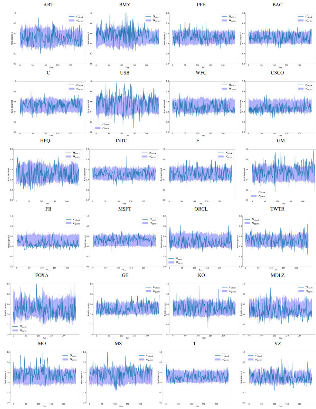
Figure 3 Evolution of Hstock and 0.1 and 0.9 quantiles of Hperm for the series of US market for τ = 1 y N = 1.

Figure 4 Evolution of Hstock and 0.1 and 0.9 quantiles of Hperm for the series of US market for τ = 5 y N = 5.
Figure 3 shows that for the US market, it is not possible in general to reject the null hypothesis Hstock = Hperm when τ = N = 1 (daily series of one-second averages), while the inspection of Fig. 4 allows concluding the existence of a clear tendency to anti-persistence (Hstock < Hperm) for τ = N = 5.
In what follows, we will focus on the latter case. Figure 5 shows for l = 300 the effect of locally shuffling the series to
destroy their short-term memory. As before, we plot Hstock and the 0.1
and 0.9 quantiles of

Figure 5 Evolution of Hstock and 0.1 and 0.9 quantiles of Hlocperm for the series of the US market for τ = 5, N = 5 y l = 300.
Once we have visually detected the general trend towards anti-persistence and the
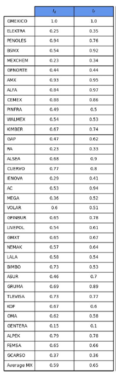
effect of local shuffling, we can define two annual inefficiency indices, one of
them given by the percentage of windows whose Hurst exponent Hstock is
below the 0.1 quantile of
To be more specific, if
then, since our data consist of 251 trading days and therefore we have 251 -N + 1 sliding N-days windows, we set Id: = Nd/(251 - N + 1). Analogously we define I f : = N f /(251 - N + 1), where
and

It is important to note that even in the case of assets with a low level of
inefficiency measured with these indices (TWTR, for example), the antipersistence
trend is clear given that the Hstock and
To formalize this idea and obtain, also here, a quantitative indicator: considering
the subset of the
Thus, this p-value indicates how likely it is to observe the behavior described above
in an efficiency scenario given by the independence between non-overlapping weekly
series. Once again, we define a strong version of this index given by

Similar results were obtained for the Mexican market (Figs. 8 and 9), although due to their lower resolution τ = 30 and N = 30 are used. It is observed that the result of the local permutations is more ambiguous in this case, which can be interpreted as short-term memory lack.

5.Conclusions
This paper discusses the efficiency in high-frequency digital markets, quantified by the Hurst exponent measured by the R/S statistic. Results indicate that, in the period from March 7, 2018, to March 7, 2019, and for the 24 assets in the United States market and the 35 in the Mexican market studied here, the Efficient Market Hypothesis is clearly rejected: the presence of long-term memory, particularly of anti-persistence, is clear.
As noted before, the relevance of these results to the question of efficiency in automated digital markets lies like our data, coming from fully-automated (algorithmic) transactions. It is because of this that we can draw the main conclusion of this paper: automated digital markets do not meet the efficiency postulated by neoclassical theory. Thus, classical explanations of the inefficiencies of human markets, based on the psychological or emotional factors of human beings 10 or their limited rationality 11, must be discarded, since the algorithms that have ordered the transactions here studied do not suffer from these human limitations. Therefore, market inefficiency seems to be due to more fundamental factors of economic dynamics. This opens a new line of investigation in the search for the real sources of the lack of efficiency.

