SciELO - Scientific Electronic Library Online

 
vol.67 número6Solutions of generalized fractional perturbed Zakharov-Kuznetsov equation arising in a magnetized dusty plasmaApplication of the modified simple equation method for solving two nonlinear time-fractional long water wave equations índice de autoresíndice de assuntospesquisa de artigos
Home Pagelista alfabética de periódicos  

Serviços Personalizados

Journal

Artigo

Indicadores

Links relacionados

  • Não possue artigos similaresSimilares em SciELO

Compartilhar


Revista mexicana de física

versão impressa ISSN 0035-001X

Rev. mex. fis. vol.67 no.6 México Nov./Dez. 2021  Epub 14-Mar-2022

https://doi.org/10.31349/revmexfis.67.060702 

Research

Gravitation, Mathematical Physics and Field Theory

Optical soliton solutions of nonlinear Davey-Stewartson equation using an efficient method

H. Günerhan1 

1Department of Mathematics, Faculty of Education, Kafkas University, Kars TR-36040, Turkey. e-mail: hatira.gunerhan@kafkas.edu.tr


Abstract

One of the most significant tools for expressing physical phenomena in the world around us is to express problems using differential equations with partial derivatives. The result of these considerations has been the invention and application of various analytical and numerical methods in solving this category of equations. In this work, we make use of a newly-developed technique called the generated exponential rational function method to compute the exact solution of the Davey-Stewartson equation. According to all the conducted research studies so far, results similar to those found in the present paper have not been published. The results attest to the efficiency of the proposed method. The method used in this paper has the ability to be implemented in other cases in solving equations with relative derivatives.

Keywords: Generalized exponential rational function method; exact soliton solutions; Davey-Stewartson equation; optical solutions; nonlinear partial differential equations

1.Introduction

Many fields of physics benefit from the nonlinear partial differential equations (NPDEs) in a wide variety of applications to mechanics, electrostatics, quantum mechanics, and finance. In linear theory, solutions usually have representation formulas and conform to the superposition principle. Despite some equations governing nature were recognized to be linear since the 19th century, this advance was widely criticized in the 20th century. It is possible to observe NPDEs not only in non-Newtonian fluids, glaciology, rheology but also in stochastic game theory, nonlinear elasticity, flow through a porous medium, and image-processing. As a result, no available superposition can be found for nonlinear equations; therefore, there is a need for studying those equations. Over the last few years, a crucial number of new methods have been proposed to obtain exact solutions for NPDEs. The Davey-Stewartson equation (DSE) has been studied in many areas of research such as chemical engineering, nonlinear mechanics, biology, and physics. To define the evolution of a three-dimensional wave packet in finite depth water, Davey-Stewartson (1974) had presented the DSE in his research study about fluid dynamics1.

In (2+1)-dimensions, the Davey-Stewartson equation is known as a solution equation that examines long and short wave resonances and other wave propagation patterns. For more details, we refer to the previous research works conducted in Refs. 2-3. The Davey-Stewartson theory is an NPDE for a complex field (wave-amplitude) q and a real field (mean flow) ϕ which is described by the following nonlinear coupled system

iqt+12(qxx+δqyy)+λ|q|2q-ϕxq=0, (1)

ϕxx-δ2ϕyy-2λ(|q|2)x=0. (1.1)

This important system of equations has attracted the attention of many researchers. For example, the line soliton 4, the semi-inverse variational principle method (SIVPM), the improved tan(ϕ/2) -expansion method (ITEM) along with the generalized G´/G-expansion method (GGM) 5, the G’/G method and the 1-soliton solution 6, the Galerkin methods 7, the extended tanh-function method 8, the generalized Kudryashov method 9, the traveling wave solutions 10, the first integral method 11, the solitary wave solution 12, the dynamical system method 13, the traveling waves solution and the exponential function method 14, the inverse scattering transform method and the soliton solutions 15, the self-similar solutions 16, the bilinear method 17,18, the single soliton and multi-soliton solutions 19, the G´/G -expansion method 20, the generalized tan(ϕ/2) method and the He’s semi-inverse variational method 21, and the bifurcation method 22,23. Others popular techniques can be found in Ref. 24,43.

In Ref. 44, Ghanbari and his collaborator developed an efficient methodology for obtaining exact solutions to NPDEs which is known as a generalized exponential rational function method (GERFM). The authors applied the technique to solve the resonant nonlinear Schrödinger equation (R-NLSE). It has been proven over time that the method enables us to be implemented in many different NPDEs arising in mathematics, physics, and engineering 45-54. The proposed method reproduces many types of precise solutions, and it is very useful for finding the exact solutions of the equation with relative ease. Recently, a new version of the method for solving partial differential equations with local fractional derivatives has been considered in Ref. 55,56.

In this paper, the GERFM is used to solve the Davey-Stewartson equation. This paper consists of the following parts: In Sec. 2, we introduce the methodology of the GERFM. In Sec. 3, the results of using the method in determining the solutions of the equation (according to the main achievement of this article) will be presented. Finally, the article ends with some concluding remarks.

2.Methodology of the GERFM

The technique is a very efficient method in solving partial differential equations 44. The basic steps of using this method are listed below.

1.NPDE will be accepted as follows:

Fu(x,t),u(x,t)x,u(x,t)t,2u(x,t)x2,=0. (2.1.)

To abbreviate the NPDEs is the following ordinary differential equation (ODE), it will be used u(ξ)=u(x,t) and ξ=kx-lt.

F(u,u',u,)=0, (2.2)

2.The crucial part of the new methodology comes from the fact that Eq.(2.2) has the formal solution of

u(ξ)=A0+k=1mAkΞ(ξ)k+k=1mBkΞ(ξ)-k, (2.3)

where

Ξ(ξ)=p1eq1ξ+p2eq2ξp3eq3ξ+p4eq4ξ. (2.4)

The real (or complex) unknown constants are A0,Ak,Bk(1km), and pk,qk(1k4). These coefficients are determined in such a way that Eq.(2.3) satisfies the nonlinear ODE of Eq. (2.2).

Also, it is essential to determine the positive integer m by the principle of balancing.

3.By adding all terms and inserting Eq. (2.3) into Eq.(2.2), the left-hand side of Eq.(2.2) is converted into the polynomial equation P(Y1,Y2,Y3,Y4)=0 in terms of Yi=eqiξ for i = 1,…,4. With the help of symbolic calculation in Maple, we obtain a set of simultaneous algebraic equations for pn,qn(1n4), and k,ω,λ,A0,A1,B1 by eliminating each coefficient of P.

4.Finally, exact solutions to Eq.(2.1.) are derived through solving the algebraic nonlinear system of equations in step 3.

3.The results

The first step is the traveling wave transformation of Eq.(1.1) by utilizing the following new variables

q=U(ξ)eiθ,ϕ=V(ξ)eiθ, (3.1)

and

ξ=iμ(x+y-ηt),θ=αx+βy+γt. (3.2)

In addition, constants of μ, η, α, and β should be determined. Using the wave transformation of Eq.(3.1) and Eq.(1.1) together with η=αδ2+βδ4, the following system of nonlinear ODE is obtained 5:

122γ+α2δ2+β2δ4U-12μ2δ21+δ2U+λU3-iμUV´=0, (3.3)

μδ2-1V´´-2iλ(U2)'=0. (3.4)

Integrating Eq. (3.4), we obtain

V=2iλμ(δ2-1)U2dξ. (3.5)

Substituting Eq.(3.5) in Eq.(3.3) will turn into the following nonlinear differential equation:

12μ2δ2(δ4-1)U+12(δ2-1)(2γ+α2δ2+β2δ4)U-λ(1+δ2)U3=0, (3.6)

where primes denote the derivatives with respect to ξ. By balancing terms of U'' and U 3 in Eq. (3.6) using homogenous principle yields 3m = m +2, so m = 1. Accordingly, the solution of Eq.(1.1) is expressed as follows:

U(ξ)=A0+A1Ξ(ξ)+B1Ξ(ξ). (3.7)

By following the described methodologies in section 2, we obtain several non-trivial solutions of (1.1).

Family 1: We attain the results for p = [1,1,-1,1] and q = [1,-1,1.-1], which gives

Ξ(ξ)=cosh(ξ)sinh(ξ). (3.8)

Case 1:

α=α, β=iα2δ4+(2A12λ-α2+2γ)δ2+2A12λ-2γδ2δ2-1,μ=λA1δδ2-1,δ=δ,γ=γ,A0=0,A1=A1,B1=0.

We have replaced the above values with Eqs. (3.7) and (3.8) together with (3.5)

U1(ξ)=A1cosh(ξ)sinh(ξ),V1(ξ)=2iλA12(ξ-coth(ξ))μ(δ2-1). (3.9)

Hence, the following exact solution was reached for Eq.(1.1):

q1(x,y,t)=(A1cosh[ξ]sinh[ξ])ei(αx+βy+γt),ϕ1(x,y,t)=(2iλA12[ξ-coth(ξ)]μ[δ2-1])ei(αx+βy+γt). (3.10)

Case 2:

α=α,β=iα2δ4+(8A12λ-α2+2γ)δ2+8A12λ-2γδ2δ2-1,μ=λA1δδ2-1,δ=δ,γ=γ,A0=0,A1=A1,B1=A1.

We have replaced the above values with Eqs. Eq.(3.7) and (3.8) together with (3.5)

U2(ξ)=(2[cosh(ξ)]2-1)A1cosh(ξ)sinh(ξ),V2(ξ)=2iλA12(4ξcosh[ξ]sinh[ξ]-2[cosh{ξ}]2+1)cosh(ξ)sinh(ξ)μ(δ2-1). (3.11)

Hence, the following exact solution has been reached for Eq.(1.1):

q2(x,y,t)=([2{cosh(ξ)}2-1]A1cosh[ξ]sinh[ξ])ei(αx+βy+γt),ϕ2(x,y,t)=(2iλA12[4ξcosh(ξ)sinh(ξ)-2\lefllcosh(ξ)\rigll2+1]cosh[ξ]sinh[ξ]μ[δ2-1])ei(αx+βy+γt). (3.12)

Case 3:

α=α,β=β,μ=i/22β2δ4+α2δ2+2γδδ2+1,δ=δ,γ=γ,A0=0,A1=0,B1=-i2δ4-1β2δ4+α2δ2+2γλ(2δ2+2).

We have replaced the above values with Eqs. (3.7) and (3.8) together with (3.5)

U3(ξ)=-i/22δ4-1β2δ4+α2δ2+2γsinh(ξ)λ(δ2+1)cosh(ξ),V3(ξ)=-i(δ4-1)(β2δ4+α2δ2+2γ)(ξ-tanh(ξ))μ(δ2-1)(δ2+1)2. (3.13)

Hence, the following exact solution has been reached for (1.1):

q3(x,y,t)=(-i/22δ4-1β2δ4+α2δ2+2γsinh(ξ)λ[δ2+1]cosh[ξ])ei(αx+βy+γt),ϕ3(x,y,t)=(-iδ4-1β2δ4+α2δ2+2γξ-tanh(ξ)μδ2-1δ2+12)ei(αx+βy+γt). (3.14)

Figure 1 shows the dynamic behavior of modulus of solutions q3x,y,t (left) and ϕ3x,y,t for δ=1.05,γ=1.3,α=β=0.5,λ=1.5, and t = 1.

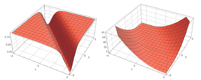
Figure 1 Dynamic behaviours modulus of solutions q3 (x; y; t) (left) and φ3 (x; y; t) (right) for δ = 1:05; γ = 1:3; a = β = 0:5; λ = 1:5; and t = 1. 

Family 2: We attain the results for p = [i,-1,1,1] and q = [i,-i,i-i], and thus one gets

Ξ(ξ)=-sin(ξ)cos(ξ). (3.15)

Case 1:

α=α,β=iα2δ4+(-8A12λ-α2+2γ)δ2-8A12λ-2γδ2δ2-1,μ=λA1δδ2-1,δ=δ,γ=γ,A0=0,A1=A1,B1=-A1.

We have replaced the above values with Eqs. (3.7) and (3.8) together with (3.5)

U4(ξ)=(2[cos(ξ)]2-1)A1sin(ξ)cos(ξ),V4(ξ)=2iλA12(-2[cos{ξ}]2-4ξcos[ξ]sin[ξ]+1)μ(δ2-1)sin(ξ)cos(ξ). (3.16)

Hence, the following exact solution has been reached for Eq.(1.1):

q4(x,y,t)=(2cos(ξ)2-1A1sin(ξ)cos(ξ) )ei(αx+βy+γt),ϕ4(x,y,t)=(2iλA12-2cos(ξ)2-4ξcos(ξ)sin(ξ)+1μδ2-1sin(ξ)cos(ξ))ei(αx+βy+γt). (3.17)

Case 2:

α=α,β=iα2δ4+(4B12λ-α2+2γ)δ2+4B12λ-2γδ2δ2-1,μ=λB1δδ2-1,δ=δ,γ=γ,A0=0,A1=B1,B1=B1.

We have replaced the above values with Eqs. (3.7) and (3.8) together with (3.5)

U5(ξ)=-B1sin(ξ)cos(ξ),V5(ξ)=2iλB12(-2[cos(ξ)]2+1)μ(δ2-1)sin(ξ)cos(ξ). (3.18)

Hence, the following exact solution has been reached for Eq.(1.1):

q5(x,y,t)=(-B1sin(ξ)cos(ξ) )ei(αx+βy+γt),ϕ5(x,y,t)=(2iλB12-2cos(ξ)2+1μδ2-1sin(ξ)cos(ξ))ei(αx+βy+γt). (3.19)

Figure 2 shows the dynamic behavior of modulus of solutions q5x,y,t (left) and ϕ5x,y,t for B1=1,δ=8.5, γ=2.01,α=4.25,λ=0.92, and t = 1.

Figure 2 Dynamic behaviours modulus of solutions q 5 (x; y; t) (left) and φ5 (x; y; t) (right) for B 1 = 1; δ= 8:5; γ = 2:01; λ = 4:25; ¸ = 0:92; and t = 1. 

Case 3:

α=α,β=iα2δ4+(-2B12λ-α2+2γ)δ2-2B12λ-2γδ2-1δ2,μ=λB1δδ2-1,δ=δ,γ=γ,A0=0,A1=0,B1=B1.

We have replaced the above values with Eqs. (3.7) and (3.8) together with (3.5)

U6(ξ)=-B1cos(ξ)sin(ξ),V6(ξ)=2iλB12(-cot(ξ)-ξ)μ(δ2-1). (3.20)

Hence, the following exact solution has been reached for equation (1.1):

q6(x,y,t)=(-B1cos(ξ)sin(ξ) )ei(αx+βy+γt),ϕ6(x,y,t)=(2iλB12[-cot(ξ)-ξ]μ[δ2-1])ei(αx+βy+γt). (3.21)

Family 3: We attain p = [1,1,-1,1 ] and q = [2,0,2,0 ], which gives

Ξ(ξ)=e2ξ+1e2ξ-1. (3.22)

Case 1:

α=α,β=iα2δ4+(8A12λ-α2+2γ)δ2+8A12λ-2γδ2-1δ2,μ=λA1δδ2-1,δ=δ,γ=γ,A0=0,A1=A1,B1=A1.

We have replaced the above values with Eqs. (3.7) and (3.8) together with (3.5)

U7(ξ)=2A1(e4ξ+1)e4ξ-1,V7(ξ)=2iλ(-4+4ξ[e4ξ-1])A12μ(δ2-1)(e4ξ-1). (3.23)

Hence, the following exact solution has been reached for Eq.(1.1):

q7(x,y,t)=(2A1[e4ξ+1]e4ξ-1)ei(αx+βy+γt),ϕ7(x,y,t)=(2iλ[-4+4ξe4ξ-1]A12μ[δ2-1][e4ξ-1])ei(αx+βy+γt). (3.24)

Case 2:

α=α,β=iα2δ4+(-4A12λ-α2+2γ)δ2-4A12λ-2γδ2-1δ2,μ=λA1δ2-1δ,δ=δ,γ=γ,A0=0,A1=A1,B1=-A1.

We have replaced the above values with Eqs. (3.7) and (3.8) together with (3.5)

U8(ξ)=4e2ξA1e4ξ-1,V8(ξ)=-8iλA12μ(δ2-1)(e4ξ-1). (3.25)

Hence, the following exact solution has been reached for Eq.(1.1):

q8(x,y,t)=(4e2ξA1e4ξ-1)ei(αx+βy+γt),ϕ8(x,y,t)=(-8iλA12μ[δ2-1][e4ξ-1])ei(αx+βy+γt). (3.26)

Figure 3 shows the dynamic behavior of modulus of solutions q8x,y,t (left) and ϕ8x,y,t for A1=1,δ=1.01,γ=2.3,α=0.2,λ=0.5, and t = 1.

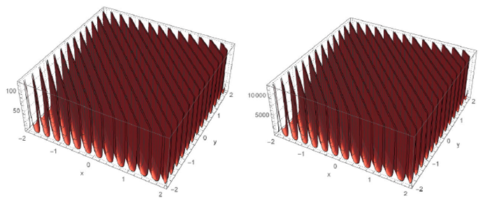
Figure 3 Dynamic behaviours modulus of solutions q 8 (x; y; t) (left) and φ8 (x; y; t) (right) for A 1 = 1; δ = 1:01; γ = 2:3; λ = 0:2; ¸ = 0:5; and t = 1. 

Family 4: We attain the results for p = [-1,3,1,-1 ] and q = [2,0,2,0 ]. So, it reads

Ξ(ξ)=-e2ξ+3e2ξ-1. (3.27)

Case 1:

α=α,β=iα2δ4+(2A12λ-α2+2γ)δ2+2A12λ-2γδ2-1δ2,μ=λA1δ2-1δ,δ=δ,γ=γ,A0=2A1,A1=A1,B1=0.

We have replaced the above values with Eqs. (3.7) and (3.8) together with (3.5)

U9(ξ)=A1(e2ξ+1)e2ξ-1,V9(ξ)=2iλ(-4+2ξ[e2ξ-1])A12μ(δ2-1)(2e2ξ-2). (3.28)

Hence, the following exact solution has been reached for equation (1.1):

q9(x,y,t)=(A1[e2ξ+1]e2ξ-1 )ei(αx+βy+γt),ϕ9(x,y,t)=(2iλ[-4+2ξ{e2ξ-1}]A12μ[δ2-1][2e2ξ-2])ei(αx+βy+γt). (3.29)

Case 2:

α=α,β=i22α2δ4+(A02λ-2α2+4γ)δ2+A02λ-4γ2δ2-1δ2,μ=A0λ2δδ2-1,δ=δ,γ=γ,A0=A0,A1=0,B1=3/2A0.

We have replaced the above values with Eqs. (3.7) and (3.8) together with (3.5)

U10(ξ)=-A0(e2ξ+3)2e2ξ-6,V10(ξ)=2iλA02(-12+2ξ[e2ξ-3])μ(δ2-1)(8e2ξ-24). (3.30)

Hence, the following exact solution has been reached for equation (1.1):

q10(x,y,t)=(-A0[e2ξ+3]2e2ξ-6)ei(αx+βy+γt),ϕ10(x,y,t)=(2iλA02[-12+2ξ{e2ξ-3}]μ[δ2-1][8e2ξ-24])ei(αx+βy+γt). (3.31)

Family 5: We attain the results for p = [-1,1,1,1 ] and q = [1,-1,1-1 ], which gives

Ξ(ξ)=-sinh(ξ)cosh(ξ). (3.32)

Case 1:

α=α,β=iα2δ4+(-4A12λ-α2+2γ)δ2-4A12λ-2γδ2-1δ2,μ=λA1δ2-1δ,δ=δ,γ=γ,A0=0,A1=A1,B1=-A1.

We have replaced the above values with Eqs. (3.7) and (3.8) together with (3.5)

U11(ξ)=A1cosh(ξ)sinh(ξ),V11(ξ)=2iλA12(-2[cosh(ξ)]2+1)μ(δ2-1)cosh(ξ)sinh(ξ). (3.33)

Hence, the following exact solution has been reached for Eq.(1.1):

q11(x,y,t)=(A1cosh(ξ)sinh(ξ))ei(αx+βy+γt),ϕ11(x,y,t)=(2iλA12[-2cosh(ξ)2+1]μ[δ2-1]cosh(ξ)sinh(ξ))ei(αx+βy+γt). (3.34)

Figure 4 shows the dynamic behavior of modulus of solutions q11x,y,t (left) and ϕ11x,y,t for A1=1,δ=1.01,γ=2.3,α=0.2,λ=0.5, and t = 1.

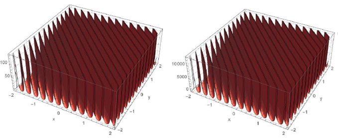
Figure 4 Dynamic behaviours modulus of solutions q 11 (x; y; t) (left) and φ11 (x; y; t) (right) for A 1 = 1; δ = 1:01; γ = 2:3; a = 0:2; λ = 0:5; and t = 1. 

Family 6: We attain the results for p = [-1-i,1-1,-1,1 ] and q = [i,-i,i-1 Α, and one obtains

Ξ(ξ)=cos(ξ)+sin(ξ)sin(ξ). (3.35)

Case 1:

α=α,β=iα2δ4+(-2A02λ-α2+2γ)δ2-2A02λ-2γδ2-1δ2,μ=A0λδ2-1δ,δ=δ,γ=γ,A0=A0,A1=0,B1=-2A0.

We have replaced the above values with Eqs. (3.7) and (3.8) together with (3.5)

U12(ξ)=A0(-sin(ξ)+cos(ξ))cos(ξ)+sin(ξ),V12(ξ)=-2iλA02(ξtan(ξ)+ξ+2)μ(δ2-1)(tan(ξ)+1). (3.36)

Hence, the following exact solution has been reached for Eq.(1.1):

q12(x,y,t)=(A0[-sin(ξ)+cos(ξ)]cos(ξ)+sin(ξ))ei(αx+βy+γt),ϕ12(x,y,t)=(-2iλA02[ξtan(ξ)+ξ+2]μ[δ2-1][tan(ξ)+1])ei(αx+βy+γt). (3.37)

Family 7: We obtain p = [-2-i,2-i,-1,1 ] and q = [i,-i,i,-i ], and thus one attains

Ξ(ξ)=cos(ξ)+2sin(ξ)sin(ξ). (3.38)

Case 1:

α=α,β=i/222α2δ4+(-A02λ-2α2+4γ)δ2-A02λ-4γδ2-1δ2,μ=1/2A0λδ2-1δ,δ=δ,γ=γ,A0=A0,A1=0,B1=-5/2A0.

We have replaced the above values with Eqs. (3.7) and (3.8) together with (3.5)

U13(ξ)=A0(-sin(ξ)+2cos(ξ))2cos(ξ)+4sin(ξ),V13(ξ)=-2iλA02(4ξtan(ξ)+2ξ+5)μ(δ2-1)(8+16tan(ξ)). (3.39)

Hence, the following exact solution has been reached for equation (1.1):

q13(x,y,t)=(A0[-sin(ξ)+2cos(ξ)]2cos(ξ)+4sin(ξ))ei(αx+βy+γt),ϕ13(x,y,t)=(-2iλA02[4ξtan(ξ)+2ξ+5]μ[δ2-1][8+16tan(ξ)])ei(αx+βy+γt). (3.40)

Family 8: We attain the results for p= [1-i,-1-i,-1,1 ] and q= [i,-i,i,-i ], and thus we obtain

Ξ(ξ)=-sin(ξ)+cos(ξ)sin(ξ). (3.41)

Case 1:

α=α,β=iα2δ4+(-2A02λ-α2+2γ)δ2-2A02λ-2γδ2-1δ2,μ=A0λδ2-1δ,δ=δ,γ=γ,A0=A0,A1=0,B1=2A0.

We have replaced the above values with Eqs. (3.7) and (3.8) together with (3.5)

U14(ξ)=2A0sin(ξ)cos(ξ)+A02(cos(ξ))2-1,V14(ξ)=-2iλA02(ξtan(ξ)-ξ+2)μ(δ2-1)(tan(ξ)-1). (3.42)

Hence, the following exact solution has been reached for Eq.(1.1):

q14(x,y,t)=(2A0sin(ξ)cos(ξ)+A02[cos(ξ)]2-1)ei(αx+βy+γt),ϕ14(x,y,t)=(-2iλA02[ξtan(ξ)-ξ+2]μ[δ2-1][tan(ξ)-1])ei(αx+βy+γt). (3.43)

Family 9: We attain the results for p= [ -3,-1,1,1 ] and q= [ 1,-1,1,-1 ], and thus we have

Ξ(ξ)=-sinh(ξ)-2cosh(ξ)cosh(ξ). (3.44)

Case 1:

α=α,β=i22α2δ4+(A02λ-2α2+4γ)δ2+A02λ-4γ2δ2-1δ2,μ=A0λ2δ2-1δ,δ=δ,γ=γ,A0=A0,A1=0,B1=3/2A0.

We have replaced the above values with Eqs. (3.7) and (3.8) together with (3.5)

U15(ξ)=A0(2sinh(ξ)+cosh(ξ))4cosh(ξ)+2sinh(ξ),V15(ξ)=2iλ(4cosh(ξ)ln(cosh(ξ)-1+sinh(ξ))+2sinh(ξ)ln(cosh(ξ)-1+sinh(ξ)))A02μ(δ2-1)(16cosh(ξ)+8sinh(ξ))+2iλ(-4cosh(ξ)ln(cosh(ξ)-1-sinh(ξ))-2sinh(ξ)ln(cosh(ξ)-1-sinh(ξ))-3sinh(ξ))A02μ(δ2-1)(16cosh(ξ)+8sinh(ξ)). (3.45)

Hence, the following exact solution has been reached for Eq. (1.1):

q15(x,y,t)=(A0[2sinh(ξ)+cosh(ξ)]4cosh(ξ)+2sinh(ξ))ei(αx+βy+γt),ϕ15(x,y,t)=V15(ξ)ei(αx+βy+γt). (3.46)

Family 10: We attain the results for p= [ -2-i,-2+i,1,1 ] and q= [ i,-i,i,-i ], and thus one has

Ξ(ξ)=sin(ξ)-2cos(ξ)cos(ξ). (3.47)

Case 1:

α=α,β=i22α2δ4+(-A02λ-2α2+4γ)δ2-A02λ-4γ2δ2-1δ2,μ=A0λ2δ2-1δ,δ=δ,γ=γ,A0=A0,A1=0,B1=5/2A0.

We have replaced the above values with Eqs. (3.7) and (3.8) together with (3.5)

U16(ξ)=A0(cos(ξ)+2sin(ξ))2sin(ξ)-4cos(ξ),V16(ξ)=-2iλA02(ξtan(ξ)-2ξ+5)μ(δ2-1)(4tan(ξ)-8). (3.48)

Hence, the following exact solution has been reached for Eq.(1.1):

q16(x,y,t)=(A0[cos(ξ)+2sin(ξ)]2sin(ξ)-4cos(ξ))ei(αx+βy+γt),\nbϕ16(x,y,t)=(-2iλA02[ξtan(ξ)-2ξ+5]μ[δ2-1][4tan(ξ)-8])ei(αx+βy+γt). (3.49)

Figure 5 shows the dynamic behavior of modulus of solutions q16x,y,t (left) and ϕ16x,y,t for A0=1,δ=1.1, γ = 0.8, α = 0.9, λ = 0.2 and t = 1.

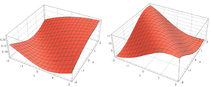
Figure 5 Dynamic behaviours modulus of solutions q 16 (x; y; t) (left) and φ16 (x; y; t) (right) for A 0 = 1; δ = 1:1; γ = 0:8; a = 0:9; λ = 0:2; and t = 1. 

Family 11: [F11] We attain the results for p= [ 1-i,1+i,1,1 ] and q= [ i,-i,i,-i ], and then one results

Ξ(ξ)=cos(ξ)+sin(ξ)cos(ξ). (3.50)

Case 1:

α=α,β=iα2δ4+(-2A12λ-α2+2γ)δ2-2A12λ-2γδ2-1δ2,μ=λA1δ2-1δ,δ=δ,γ=γ,A0=-A1,A1=A1,B1=0,

We have replaced the above values with Eqs. (3.7) and (3.8) together with (3.5)

U17(ξ)=A1sin(ξ)cos(ξ),V17(ξ)=2iλA12(tan(ξ)-ξ)μ(δ2-1). (3.51)

Hence, the following exact solution was reached for Eq. (1.1):

q17(x,y,t)=(A1sin(ξ)cos(ξ))ei(αx+βy+γt),ϕ17(x,y,t)=(2iλA12[tan(ξ)-ξ]μ[δ2-1])ei(αx+βy+γt). (3.52)

Figure 6 shows the dynamic behavior of modulus of solutions q17x,y,t (left) and ϕ17x,y,t for A1=1,δ=1.5,γ=0.5, α = 0.1, λ = 0.2 and t = 1.

Figure 6 Dynamic behaviours modulus of solutions q 17 (x; y; t) (left) and φ17 (x; y; t) (right) for A 1 = 1; δ = 1:5; γ = 0:5; a = 0:1; λ = 0:2; and t = 1. 

Family 12:

We attain the results for p= [ -3,-2,1,1 ] and q= [ 0,1,0,1 ], and we get

Ξ(ξ)=-3-2eξ1+eξ. (3.53)

Case 1:

α=α,β=i/525α2δ4+(2A02λ-25α2+50γ)δ2+2A02λ-50γδ2-1δ2,μ=2A0λ5δ2-1δ,δ=δ,γ=γ,A0=A0,A1=0,B1=12A05,

We have replaced the above values with Eqs. (3.7) and (3.8) together with (3.5)

U18(ξ)=-A02eξ-315+10eξ,V18(ξ)=2iλA02(2ξeξ+3ξ+12)μ(δ2-1)(75+50eξ). (3.54)

Hence, the following exact solution has been reached for equation (1.1):

q18(x,y,t)=(-A0[2eξ-3]15+10eξ)ei(αx+βy+γt),ϕ18(x,y,t)=(2iλA02[2ξeξ+3ξ+12]μ[δ2-1][75+50eξ])ei(αx+βy+γt). (3.55)

Figure 7 shows the dynamic behavior of modulus of solutions q18x,y,t (left) and ϕ18x,y,t for A0=1,δ=5, γ = 0.1, α = 1.5, λ = 0.3 and t = 1.

Figure 7 Dynamic behaviours modulus of solutions q 18 (x; y; t) (left) and φ18 (x; y; t) (right) for A 1 = 1; δ = 5; γ = 0:1; a = 1.5; λ = 0:3; and t = 1. 

Family 13:

We attain the results for p= [ -1,-2,1,1 ] and q= [ 1,0,1,0 ], and one finds

Ξ(ξ)=-eξ-2eξ+1. (3.56)

Case 1:

α=α,β=i9α2δ4+(2A02λ-9α2+18γ)δ2+2A02λ-18γ3δ2-1δ2,μ=2A0λ3δ2-1δ,δ=δ,γ=γ,A0=A0,A1=0,B1=4/3A0.

We have replaced the above values with Eqs. (3.7) and (3.8) together with (3.5)

U19(ξ)=-A0(eξ-2)3eξ+6,V19(ξ)=2iλA02(ξeξ+2ξ+8)μ(δ2-1)(9eξ+18). (3.57)

Hence, the following exact solution has been reached for equation (1.1):

q19(x,y,t)=(-A0[eξ-2]3eξ+6)ei(αx+βy+γt),ϕ19(x,y,t)=(2iλA02[ξeξ+2ξ+8]μ[δ2-1][9eξ+18])ei(αx+βy+γt). (3.58)

Family 14: We attain the results for p= [ 2,1,1,1 ] and q= [ 1,0,1,0 ], and then we obtain

Ξ(ξ)=2eξ+1eξ+1. (3.59)

Case 1:

α=α,β=i9α2δ4+(2A02λ-9α2+18γ)δ2+2A02λ-18γ3δ2-1δ2,μ=2A0λ3δ2-1δ,δ=δ,γ=γ,A0=A0,A1=0,B1=-4/3A0.

We have replaced the above values with Eqs. (3.7) and (3.8) together with (3.5)

U20(ξ)=A0(2eξ-1)6eξ+3,V20(ξ)=2iλA02(2ξeξ+ξ+4)μ(δ2-1)(18eξ+9). (3.60)

Hence, the following exact solution has been reached for equation (1.1):

q20(x,y,t)=(A0[2eξ-1]6eξ+3)ei(αx+βy+γt),ϕ20(x,y,t)=(2iλA02[2ξeξ+ξ+4]μ[δ2-1][18eξ+9])ei(αx+βy+γt). (3.61)

Family 15: We attain the results for p= [ -1,0,1,1 ] and q= [ 0,0,1,0 ], and then we find

Ξ(ξ)=-11+eξ. (3.62)

Case 1:

α=iβ2δ6-β2δ4+(2A02λ+2γ)δ2+2A02λ-2γδ2-1δ,β=β,μ=2A0λδδ2-1,δ=δ,γ=γ,A0=A0,A1=2A0,B1=0.

We have replaced the above values with Eqs. (3.7) and (3.8) together with (3.5)

U21(ξ)=A0(eξ-1)1+eξ,V21(ξ)=2iλA02(ξeξ+ξ+4)μ(δ2-1)(1+eξ) (3.63)

Hence, the following exact solution has been reached for equation (1.1):

q21(x,y,t)=(A0[eξ-1]1+eξ)ei(αx+βy+γt),ϕ21(x,y,t)=(2iλA02[ξeξ+ξ+4]μ[δ2-1][1+eξ])ei(αx+βy+γt). (3.64)

Figure 8 shows the dynamic behavior of modulus of solutions q21x,y,t (left) and ϕ21x,y,t for A0=1,δ=2,γ=0.9,β=0.5,λ=0.7, and t = 1.

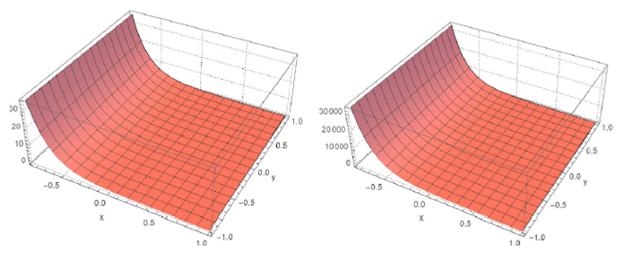
Figure 8 Dynamic behaviours modulus of solutions q 21 (x; y; t) (left) and φ21 (x; y; t) (right) for A 0 = 1; δ = 2; γ = 0:9; β = 0.5; λ = 0:7; and t = 1. 

Remark 1 In each of the above cases, we take ξ=iμx+y-αδ2+βδ4t.

4.Conclusion

Partial differential equations have many applications in modeling practical problems in our lives. This importance has created additional motivation for researchers to develop new and efficient methods. Some of these techniques enable us to achieve exact solutions to such problems. However, determining such solutions is impossible or very difficult for some categories of equations. The method used in this paper, called the GERFM, is a powerful technique to determine the exact solutions to different types of PDEs. In this survey, the method has been utilized to solve the Davey-Stewartson equation. It was shown that the method is a suitable technique to solve the Davey-Stewartson equation with this study. The results are quite reliable for solving this problem. Further, we believe that the presented methods and results in this paper are valuable to all researchers in the field of mathematical physics. Therefore, GERFM offers an excellent opportunity for future research studies on related topics of the research. This emphasizes the power of the method used in providing exact solutions to various real-world applied models.

References

1. A. Davey, K. Stewartson, On three-dimensional packets of surface waves, Proc. R. Soc. London Ser. A, 338 (1974) 101. https://doi.org/10.1098/rspa.1974.0076. [ Links ]

2. C. Babaoglu, Long-wave short-wave resonance case for a generalized Davey-Stewartson system, Chaos Solitons Fractal 38 (2008) 48. https://doi.org/10.1016/j.chaos.2008.02.007. [ Links ]

3. K.W. Chow, S.Y. Lou, Propagating wave patterns and peakons of the Davey-Stewartson system, Chaos Solitons Fractal, 27 (2006) 561. https://doi.org/10.1016/j.chaos.2005.04.036. [ Links ]

4. M. D. Groves, S-M Sun, E. Wahln, Periodic solitons for the elliptic-elliptic focussing Davey-Stewartson equations, C. R. Math. 354 (2016) 486. https://doi.org/10.1016/j.crma.2016.02.005. [ Links ]

5. R. F. Zinati and J. Manafian, Applications of He’s semi-inverse method, ITEM and GGM to the Davey-Stewartson equation, Eur. Phys. J. Plus. 132 (2017) 155. https://doi.org/10.1140/epjp/i2017-11463-3. [ Links ]

6. G. Ebadi and A. Biswas, The G0=G method and 1-soliton solution of the Davey-Stewartson equation, Math. Comput. Model. 53 (2011) 694. https://doi.org/10.1016/j.mcm.2010.10.005. [ Links ]

7. Y. Gao, L. Mei, R. Li, Galerkin methods for the Davey-Stewartson equations, Appl. Math. Comput. 328 (2018) 144. https://doi.org/10.1016/j.amc.2018.01.044. [ Links ]

8. L. Chang, Y. Pan, X. Ma, New exact travelling wave solutions of Davey-Stewartson equation, J. Comput. Inf. Syst. 9 (2013) 1687. [ Links ]

9. S. Tuluce Demiray, H. Bulut, New soliton solutions of Davey-Stewartson equation with power-law nonlinearity, Opt. Quant. Electron. 49 (2017) 117. https://doi.org/10.1007/s11082-017-0950-6. [ Links ]

10. M. Song, A. Biswas , Topological defects and bifurcation analysis of the DS equation with power law nonlinearity, Appl. Math. Inf. Sci. 9 (2015) 1719. [ Links ]

11. H. Jafari, A. Sooraki, Y. Talebi, A. Biswas, The first integral method and traveling wave solutions to Davey-Stewartson equation, Nonlinear Anal. Model. Control, 17 (2012) 182. https://doi.org/10.15388/NA.17.2.14067. [ Links ]

12. O.H. El-Kalaawy, R.S. Ibrahim, Solitary wave solution of the two-dimensional regularized long-wave and Davey-Stewartson equations in fluids and plasmas, Appl. Math. 3 (2012) 833.https://doi.org/10.4236/am.2012.38124. [ Links ]

13. G. Ebadi, E.V. Krishnan, M. Labidi, E. Zerrad, A. Biswas -Analytical and numerical solutions to the Davey-Stewartson equation with power-law nonlinearity, Wave Random Complex Media 21 (2011) 559. https://doi.org/10.1080/17455030.2011.606853. [ Links ]

14. J. Shi, J. Li, S. Li, Analytical travelling wave solutions and parameter analysis for the (2+1)-dimensional Davey-Stewartsontype equations, Pramana J. Phys. 81 (2013) 747. https://doi.org/10.1007/s12043-013-0612-6. [ Links ]

15. V. A. Arkadiev, A. K. Pogrebkov, and M.C. Polivanov, Inverse scattering transform method and soliton solutions for the Davey-Stewartson II equation, Phys. D 36 (1989) 189. https://doi.org/10.1016/0167-2789(89)90258-3. [ Links ]

16. X. Zhao, Self-similar solutions to a generalized Davey-Stewartson system, Math. Comput. Model. 50 (2009) 1394 ,https://doi.org/10.1016/j.mcm.2009.04.023. [ Links ]

17. Y. Ohta and J. Yang, Dynamics of rogue waves in the Davey-Stewartson II equation, J. Phys. A 46 (2013) 105202. https://doi.org/10.1088/1751-8113/46/10/105202. [ Links ]

18. Y. Ohta and J. Yang, Rogue waves in the Davey-Stewartson I equation, Phys. Rev. A Math. Theor. 86(2012)036604. https://doi.org/10.1103/PhysRevE.86.036604. [ Links ]

19. D. Anker and N.C. Freeman, On the Solition Solutions of the Davey-Stewartson Equation for Long Waves, Proc. R. Soc. Lond. A. 360(1978) 529. https://doi.org/10.1098/rspa.1978.0083. [ Links ]

20. B. Zhang, M.N. Xiong, L. Chen, Many New Exact Solutions for Generalized Davey-Stewartson Equation with Arbitrary Power Nonlinearities Using Novel (G0=G)-Expansion Method, J. Adv. Appl. Math. 4 (2019) 10. https://doi.org/10.22606/jaam.2019.41002. [ Links ]

21. M. Fazli Aghdaei, H. Adibi, New methods to solve the resonant nonlinear schrödinger equation with time-dependent coefficients, Opt. Quantum Electronics 49 (2017) 316. https://doi.org/10.1007/s11082-017-1152-y. [ Links ]

22. M. Song, Z.R. Liu, ”Qualitative analysis and explicit traveling wave solutions for the Davey-Stewartson equation, Math. Methods Appl. Sci. 37 (2014) 393. https://doi.org/10.1002/mma.2798. [ Links ]

23. J. Cao, H.Y. Lu, Exact traveling wave solutions of the generalized Davey-Stewartson equation, J. Shanghai Norm. Univ. 44 (2015) 330. [ Links ]

24. K. Munusamy, C. Ravichandran, K. S. Nisar and B. Ghanbari, Existence of solutions for some functional integrodifferential equations with nonlocal conditions, Math. Methods Appl. Sci. 43 (2020) 10319. https://doi.org/10.1002/mma.6698. [ Links ]

25. G. Rahman, K. S. Nisar, B. Ghanbari, and T. Abdeljawad, On generalized fractional integral inequalities for the monotone weighted Chebyshev functionals, Adv. Differ.Equ. 2020 (2020) 368. https://doi.org/10.1186/s13662-020-02830-7. [ Links ]

26. M. Eslami and H. Rezazadeh, The first integral method for Wu-Zhang system with conformable time-fractional derivative, Calcolo53 (2016) 475. https://doi.org/10.1007/s10092-015-0158-8. [ Links ]

27. R. M. Jena Rajarama, S. Chakraverty, H. Rezazadeh, and D. Domiri Ganji, On the solution of time-fractional dynamical model of Brusselator reaction-diffusion system arising in chemical reactions, Mathematical Methods in the Applied Sciences 43 (2020) 3903. https://doi.org/10.1002/mma.6141. [ Links ]

28. M. Inc et al., New solitary wave solutions for the conformable Klein-Gordon equation with quantic nonlinearity, AIMS Math. 5 (2020) 6972. https://doi.org/10.3934/math.2020447. [ Links ]

29. M. Inc, M. Miah, A. Akher Chowdhury Shahadat, H. Rezazadeh, M.A. Akinlar, Y.M. Chu, New exact solutions for the Kaup-Kupershmidt equation, AIMS Math., 5 (2020) 6726. https://doi.org/10.3934/math.2020432. [ Links ]

30. A. C. Cevikel, A. Bekir, S. San, M. B. Gucen, Construction of periodic and solitary wave solutions for the complex nonlinear evolution equations, J. Franklin Inst. 351 (2014) 694. https://doi.org/10.1016/j.jfranklin.2013.04.017. [ Links ]

31. A. C. C¸ evikel, A. Bekir, M. Akar, S. San, A procedure to construct exact solutions of nonlinear evolution equations, Pramana 79 (2012) 337. https://doi.org/10.1007/s12043-012-0326-1. [ Links ]

32. A. Bekir , A. C. Cevikel , New solitons and periodic solutions for nonlinear physical models in mathematical physics, Nonlinear Anal. Real World Appl. 11 (2010) 3275. https://doi.org/10.1016/j.nonrwa.2009.10.015. [ Links ]

33. A. Bekir and A. C. Cevikel, Solitary wave solutions of two nonlinear physical models by tanh-coth method, Commun. Nonlinear Sci. Numer. Simul. 14 (2009) 1804. https://doi.org/10.1016/j.cnsns.2008.07.004. [ Links ]

34. A. C. Çevikel and A. Bekir, New solitons and periodic solutions for (2+1)-dimensional Davey-Stewartson equations, Chin. J. Phys., 51 (2013) 1. https://doi.org/10.6122/CJP.51.1. [ Links ]

35. A. Bekir and A. C. C¸ Çevikel, New exact travelling wave solutions of non-linear physical models, Chaos Solitons Fractals 41(2009) 1733. https://doi.org/10.1016/j.chaos.2008.07.017. [ Links ]

36. A. Bekir, A. C. Çevikel, O. Guner, S. San, Bright and Dark Soliton Solutions of the (2+1)-Dimensional Evolution Equations, Math. Model. Anal. 19(2014) 118. https://doi.org/10.3846/13926292.2014.893456. [ Links ]

37. Ö . Güner, A. Bekir, and A. C. Çevikel, Dark soliton and periodic wave solutions of nonlinear evolution equations, Adv. Differ. Equ. 2013 (2013) 68. https://doi.org/10.1186/1687-1847-2013-68. [ Links ]

38. A. C. Çevikel, New Exact Solutions of The Space-Time Fractional KdV-Burgers and Non-Linear Fractional Foam Drainage Equation, Therm. Sci. 22 (2018) 15. https://doi.org/10.2298/TSCI170615267C. [ Links ]

39. A. Bekir, O. Guner, A. C. Çevikel, The Exp-function Method for Some Time-fractional Differential Equations, IEEE/CAA J. Autom. Sinica 4 (2017) 315. https://doi.org/10.1109/JAS.2016.7510172. [ Links ]

40. A. Bekir, O. Guner, A. Burcu, A. C. C¸ Çevikel, Exact Solutions for Fractional Differential-Difference Equations by (G/G)-Expansion Method with Modified Riemann-Liouville Derivative, Adv. Appl. Math. Mech. 8 (2016) 293. https://doi.org/10.4208/aamm.2014.m798. [ Links ]

41. E. Aksoy, A. Bekir, A. C. Çevikel, Study on Fractional Differential Equations with Modified Riemann-Liouville Derivative via Kudryashov Method, Int. J. Nonlinear Sci. Numer. Simul. 20(2019) 511. https://doi.org/10.1515/ijnsns-2015-0151. [ Links ]

42. H. Günerhan, Exact traveling wave solutions of the Gardner equation by the improved tan(£(#))-expansion method and the wave ansatz method, Math. Probl. Eng. 2020 (2020) 5926836, https://doi.org/10.1155/2020/5926836. [ Links ]

43. H. Dutta, H. Günerhan, K.K. Ali, R. Yilmazer, Exact Soliton Solutions to the Cubic-Quartic Non-linear Schrödinger Equation With Conformable Derivative, Front. Phys., 8 (2020) 62. https://doi.org/10.3389/fphy.2020.00062. [ Links ]

44. B. Ghanbari and M. Inc, A new generalized exponential rational function method to find exact special solutions for the resonance nonlinear Schrödinger equation, Eur. Phys. J. Plus 133 (2018) 142. https://doi.org/10.1140/epjp/i2018-11984-1. [ Links ]

45. B. Ghanbari and J.F. Gómez-Aguilar, The generalized exponential rational function method for Radhakrishnan-Kundu-Lakshmanan equation with β-conformable time derivative, Rev. Mex. Fis. 65 (2019) 503. https://doi.org/10.31349/RevMexFis.65.503. [ Links ]

46. H.M. Srivastava, H. Günerhan, B. Ghanbari, Exact travelingwave solutions for resonance nonlinear Schrödinger equation with intermodal dispersions and the Kerr law nonlinearity, Math Meth Appl Sci., 42 (2019) 7210. https://doi.org/10.1002/mma.5827. [ Links ]

47. B. Ghanbari, H. Günerhan, O.A. ´Ihan, and H.M. Baskonus, Some new families of exact solutions to a new extension of nonlinear Schrödinger equation, Phys. Scr. 95 (2020) 075208. https://doi.org/10.1088/1402-4896/ab8f42. [ Links ]

48. B. Ghanbari and C-Ku. Kuo, A variety of solitary wave solutions to the (2+1)-dimensional bidirectional SK and variable coefficient SK equations, Results in Physics 18 (2020) 103266. https://doi.org/10.1016/j.rinp.2020.103266. [ Links ]

49. B. Ghanbari, M. Incand L. Rada, Solitary wave solutions to the Tzitzeica type equations obtained by a new efficient approach, J. Appl. Anal. Comput. 9(2018) 568. https://doi.org/10.11948/2156-907X.20180103. [ Links ]

50. B. Ghanbari, H. Günerhan, S. Momani, Exact optical solutions for the regularized long-wave Kadomtsev-Petviashvili equation, Phys. Scr. 95 (2020) 105208. https://doi.org/10.1088/1402-4896/abb5c8. [ Links ]

51. B. Ghanbari, K. S. Nisar, and M. Aldhaifallah, Abundant solitary wave solutions to an extended nonlinear Schrödinger’s equation with conformable derivative using an efficient integration method, Adv. Differ. Eq. 2020 (2020) 328. https://doi.org/10.1186/s13662-020-02787-7. [ Links ]

52. M. S. Osman, B. Ghanbari, and J. A. T. Machado, New complex waves in nonlinear optics based on the complex Ginzburg-Landau equation with Kerr law nonlinearity, Eur.Phys. J. Plus. 134 (2019) 20. https://doi.org/10.1140/epjp/i2019-12442-4. [ Links ]

53. B. Ghanbari, A. Yusuf, and D. Baleanu, The new exact solitary wave solutions and stability analysis for the(2+1)-dimensional Zakharov-Kuznetsov equation, Adv. Differ. Eq., 2019 (2019) 49. https://doi.org/10.1186/s13662-019-1964-0. [ Links ]

54. S. Kumar, A. Kumar, A-M Wazwaz, New exact solitary wave solutions of the strain wave equation in microstructured solids via the generalized exponential rational function method, Eur. Phys. J. Plus 135(2020) 1. [ Links ]

55. B. Ghanbari, On novel non-differentiable exact solutions to local fractional Gardner’s equation using an effective technique, Math. Methods Appl. Sci. (2020) 4673. https://doi.org/10.1002/mma.7060. [ Links ]

56. B. Ghanbari, On the non-differentiable exact solutions to Schamel’s equation with local fractional derivative on Cantor sets, Numer. Methods Partial Differ. Equ. (to be published), https://doi.org/10.1002/num.22740. [ Links ]

Received: December 29, 2020; Accepted: January 23, 2021

Creative Commons License This is an open-access article distributed under the terms of the Creative Commons Attribution License