nova página do texto(beta)
 Inglês (pdf)
 Artigo em XML
 Referências do artigo
 Enviar este artigo por email
 Citado por SciELO
  Similares em
SciELO
Similares em
SciELO 
 Permalink
1. Introduction
The epidemics of Covid-19 has prompted a lot of researchers from different fields to use their diverse expertise to understand the nature of the Sars-Cov-2 virus and its spreading worldwide. In particular, out of the medical sciences, the epidemics have revealed a rich ground where physicists, mathematicians, and statisticians are eager to apply their knowledge and contribute to its amelioration and containment at the local and global stages.
From the formal point of view, there has been much research in the so-called epidemic models and their mathematical properties, see for instance [1,2], being the compartmental models the most widely used and studied. In general, the models consider the classification of a given population in some parts: Susceptible (S), Infective (I), Recovered (R), among others, and are then dubbed in terms of which of them they consider for the dynamics of the disease: SIR, SEIR, etcetera. There is historical evidence that such models are in good agreement with the dynamics of past epidemics [1], and such past successes have triggered its use in the present crisis, see for instance, [3-11].
However, there is an inherent difficulty in studying the Covid-19 epidemics in real-time: that data collection is not perfect and, in most cases, is certainly incomplete and not very useful to fully characterize the evolution of the epidemics [12,13]. One then must question whether the use of very complex models is convenient, given the scarcity and flaws of the data series. Actually, it seems that simple models are sufficient to understand the epidemics [14,15].
Given the above considerations, here we study the simplest of compartmental models and use them for the description of the current epidemics in different countries. The model only accounts for two parts of the population: Susceptibles and Infectives, and is known as the SI model. The infectives in the model are not supposed to recover, and then its number is an ever-increasing function of time, which is what one sees in the daily reports of cumulative infectives released by health authorities worldwide. In this respect, the SI model seems to be a convenient one to follow the evolution of the real data at hand.
However, the original SI model has one free parameter, the transmission rate, which is assumed to be a constant parameter, but this seems to be an oversimplification that is not in agreement with real data. This has inspired the use of timedependent transmission rates, which expand the capabilities of the compartmental models to encompass hidden complexities of the data compilations. Here we take this point of view and consider a time-dependent transmission rate in terms of an exponentially decreasing function, as it was done first in [16], and also in Ref. [17] (see also [18,19] for other examples). Additionally, we also take into account the data series of cumulative deaths, using simple assumptions without extending the SI model, which is thought to be at least as reliable as those of cumulative infectives, and probably a better representation of the epidemic’s course [14].
A summary of the paper is as follows. In Sec. 2, we present the mathematical description of the standard SI model, which we call the time-independent version, and give a brief account of its main properties. We then explain its generalization to accommodate a time-dependent transmission rate and find the analytical solution in terms of a logistic function for the general case. It is argued that, because of the time-dependence of the transmission rate, the total population number can be freely chosen, and there is a simpler, approximated solution of the time-dependent SI system in the limit of a large population number in the form of a Gompertz function [20,21]. Using real data, we look for evidence of a time-dependent transmission rate in terms of its definition within the SI system, and then we propose an exponential-like parametrization of the transmission rate.
In Sec. 3, we use the time-dependent models of Sec. 2 and use them to make a fitting of their free parameters to data from some chosen countries. The fit is made using the Bayesian inference, and the results are giving an interpretation in terms of characteristic quantities and times that are intrinsic to our parametrized transmission rate. Finally, the main conclusions of our study and future perspectives are summarized in Sec. 4.
2. Mathematical background
Here we present the main mathematical expressions for the time-dependent epidemic model, based on the known compartmental model SI.
2.1. Time-independent SI
The SI model is represented by the following set of equations,
Here, S(I) is the number of susceptible (infectious) people, the total population is N = S+I, β is the infection rate (i.e., the probability per unit time that an individual contracts the disease), and a dot means derivative for time. i
Because of the conservation equation, the SI system is truly one-dimensional and represented by the equation,
If β is a constant parameter, the solution of Eq. (2) is the sigmoid, also known as the logistic function [22],
where t 0 is an integration constant.
From the second derivative of Eq. (3) (the first derivative of Eq. (2)),
Then, there is a maximum of the first derivative at t = t 0, which also corresponds to an inflection point of the logistic function (Ï= 0) at which I = N/2. As for the logistic function itself, notice that the initial and asymptotic values of the logistic function (3) are, respectively,
In other words, the saturation value of the infectious people is the whole of the available population. If N is a large number, and for the same I i , the only change is the position of the inflection point t 0, which shifts to larger values.
2.2. Time-dependent SI system
Let us now consider the case of a time-dependent infection rate, that is, β = β(t). Notice that we do not need to change the nature of the original SI system (1), and then we can use again Eq. (2) to find a solution to a time-dependent SI system. It can be readily shown that the solution can be written as a generalized logistic function [21,23] (see also [24]),
where u 0 is an integration constant. Notice that Eq. (6a) is again the sigmoid function but only now in terms of a new variable u. The initial and asymptotic values of the infected people are given by
Here, u ∞ = u(t → ∞), which may or may not be a finite value, and this depends on the chosen function β, see Eq. (6a).
Notice that the second derivative of Eq. (2) for a timedependent transmission rate is
Hence, the true inflection point Ï = 0 does not correspond to I = N/2 anymore as it was in the time-independent case. However, it can be shown that the time-independent SI solution (3) is a particular case of the time-dependent one (6a). In the case β = const., one readily obtains that u(t) = βt, and then Eq. (3) is recovered if also u 0 = βt 0.
The exact solution (6a) opens up the possibility to consider the evolution of a disease in which the transmission rate is changing, whether by natural means or by human intervention. This is a more realistic approach, and it has the advantage that we can continue dealing with the accumulated numbers reported by the health systems worldwide.
2.3. The large N limit
In the time-independent SI system, the constant of integration is fixed by the initial conditions and the total population number, namely e βt0 = N/I i − 1, and then the asymptotic value of the infectives is the total population, see Eqs. (5). However, in the time-dependent case, the asymptotic value of infectives also depends on the asymptotic value u ∞, which means that not all the population will get infected, that is, I ∞ < N.
The ratio between the total and the initial number of infectives can be written as
Here, u ∞ is an independent constant, and then one can obtain the same ratio by adjusting accordingly the values of u 0 and u ∞. In this sense, there is a new degeneracy in the time-dependent system as the total number of infectives is not uniquely determined by the total population number N. Explicitly, the degeneracy reads
If we keep the ratio (I ∞ /I i ) fixed, we obtain that
The final ratio of infectives, in this limit, can be calculated directly from the asymptotic value of the variable u. Given that e u0 = N/I i − 1, we call this the large N limit.
Actually, one can do the same exercise in the general expression of infectives. If we write Eq. (6a) (see also Eq. (6b)) in the form,
we find that for large enough values of u 0, i.e., N → ∞, the function of infectives can be approximated as
The evolution of the disease is simply driven by the transmission rate, and then the asymptotic limit is obtained if the integral on the rhs of (11a) converges for t → ∞. Actually, the ratio between the asymptotic and initial values of infectives is
which is in turn the same result as in Eq. (9) above.
The expression (11a) gives a simplified evolution of the disease. For instance, the first derivative is just I
˙ = βI, whereas the second derivative is Ï = (
There is a small warning here about the parametrization of β. If we assume that the transmission rate is given by β = β(t,k ` ), where k ` are in general constant parameters, one must be aware that their values will depend on N, and then the values obtained from Eq. (11a) are not the same as those from Eq. (10). They will, in both cases, deliver the same values of I i and I ∞, but the evolution profile I(t) will have some differences in the two cases.
2.4. Time-dependent β from real data
One important question is whether real data suggest a complex evolution of the Covid-19 disease, for which the simple time-independent SI system would be insufficient to describe it. To get an answer directly from the data available, we make use here of an analytical result that can be derived from the general case (6a).
First, we write down the following expression to define the time-dependent function Γ(t),
which is valid for any form of β and is directly derived from Eqs. (6); it is also valid for the large N approximation (11a). In the time-independent case, for which I ∞ = N, we readily obtain Γ(t) = β = const. But in the general case, we find at t = 0 that
Another characteristic value is found at late times, as u → u ∞. In this case, we use the approximation 1 − e u−u∞ ≃ u −u ∞, and then from Eq. (6a), we obtain that
if such limit exists.
Thus, the function Γ(t) can help us to decide whether to use the time-independent or the time-dependent SI system, as the expression (12a) can be easily calculated from data in countries that already show an asymptotic value of infectives. In Fig. 1, we show data from Mexico, ii which is one of the countries that comply with the preceding condition, as seen on the left panel for the number of positives normalized to the latest reported value (the first day in the time series is that of the first registered death). Shown also is the evolution of reported deaths, which is too normalized to the value of the latest reported value.
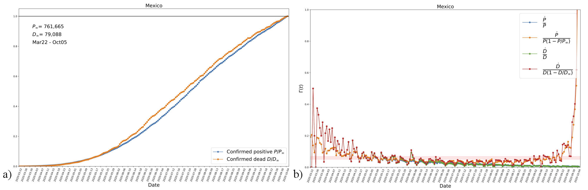
FIGURE 1 a) Data from Mexico showing the evolution of accumulated confirmed positives and deaths, the time series starts at the date of the first registered death (from March 22 until October 5). The values in the plot are normalized with their respective last data point. It can be noticed that both quantities seem to have reached an asymptotic final value. b) The estimated evolution of function Γ(t), see Eq. (12a), according to data of new daily cases for both confirmed positives and deaths. Shown are three different combinations of each data compilation, where P ∞ and D ∞ are the last data points in the corresponding time series. The trends of the three cases suggest a decrease in the transmission rate β with time. The orange-shaded horizontal region (with vertical range 0.05 − 0.07) is just shown for reference. See Sec. 2.4. and the text for more details
On the right panel of Fig. 1, we see the daily new cases (with the same mentioned normalization) divided by different combinations of accumulated numbers. In the plots P, (D) refers to confirmed positives (deaths). Notice that the combinations in the plot represent the function (12a), and then data seems to indicate that Γ(t) is a decreasing function that approaches a constant value at late times. In contrast, when we use the expression İ/I , the ratio goes to zero. Our interpretation is that data suggest a time-dependent transmission rate β, particularly one that decays with time. Although we only show the case of Mexico, we have found the same trend in all cases in which data already shows an asymptotic value of accumulated positives (e.g., Germany, France, and others).
It is clearly seen that β is, in general, a decaying function as time proceeds, which in our opinion is a manifestation of governmental intervention to slow the spread of the disease. Although there is not a unique function, given the profile suggested in Fig. 1, we will consider an exponentially decaying function as an approximation to the evolution of β. That is, we write it explicitly as
where k 0 ,k 1 are constant parameters. The corresponding time variable in Eq. (6a) is
and then for this case, we see that u ∞ = k 0 /k 1.
In limit k 1 t≪ 1, we obtain that u(t) ≃k 0 t, , which is the expected behavior in the time-independent case. Then, k 0 determines the initial growth of the epidemics, whereas k 1 gives the decay time of the transmission rate, with a half-life time given by t 1/2 = ln2/k 1.
Likewise, the asymptotic value of the infectives is I ∞ = I i e k0/k1 , see Eqs. (9) and (11b), and then the ratio between the asymptotic and initial values will depend on the ratio k 0 /k 1. Here we see the importance of k 1: the smaller its value, the larger it takes for the epidemics to fade away and the larger the asymptotic value of total infectives.
As for the time-dependent function Γ(t) defined in Eq. (12a), after using Eqs. (13) we find that
Notice that Eq. (14) is also in agreement with the expectation from data in Fig. 1: there are well definite values of Γ(t) at early and late times at late times, where the value at late times will give us an indication of the decay time of the transmission rate β.
We mentioned before that it is impossible to have an analytical expression for the inflection time of the sigmoid function (6a) for a general β(t). However, one can instead write an expression for the time at which the infected population I(t 50) is one-half (50%) of the asymptotic value, i.e., I(t 50) = I ∞ /2. After some straightforward algebra using Eqs. (6), we find in general for the generalized time variable that
Hence, from the particular parametrization (13a), we finally obtain
We will use t 50 as a point of reference in the time series of the different data in our analysis below, similar to the inflection point of the standard sigmoid function. Another useful point is that at which the number of infectives is 90% of the asymptotical value, I(t 90) = 0.9I ∞, as it can be considered as a reference for the upcoming end of the infection period. Following the same calculations that led to Eqs. (15), we find
and its corresponding time, again for the particular parametrization (13a), is
3. Statistical analysis and results
Our main assumption is that the time series of both confirmed positives and deaths have a common origin from the total number of infected people I(t). Formally speaking, we are assuming that
where r P is the fraction of infected people that are tested and confirmed as positive, whereas r D is the fraction of infected people that is confirmed positive and eventually pass away. Notice that we consider that D(t) evolves with a time delay t D for I(t) (and also to P(t)). Such delay is difficult to measure reliably, and here, we will report the values suggested by the data itself.
In the following sections, we do the fitting to data using two different models. The first one, which we call model A, considers the generalized logistic function (6a) and the parametrization (13a) of the transmission rate. The second one, which we dub model B, uses the large N approximation represented by Eq. (11a) and the same parametrization of the transmission rate. As discussed previously in Sec. 2.4, data seems to discard the time-independent SI system, but for completeness, we also report its fitting to data in Appendix C.
3.1. Model A and fitting to data
We will consider the following parametrization of the logistic function of the confirmed positive people, in cumulative numbers,
Following the discussion at the beginning of this section, we will also consider the reports of accumulated deaths, which we assume to follow a similar logistic function as those of the confirmed positive, except for a different amplitude and inflection point,
Our model then has seven free parameters: P
0, D
0, t
D
, u
0,
We will assume that the data provided follows the trend of the real number of infected people and deaths and that both of these numbers will eventually reach a saturation value soon as has happened in past diseases. Moreover, as we do not know the systematic errors in the processing of the data, we will assume some level of intrinsic error by using a Poisson distribution. To ease the fitting of data from different countries, we normalize the data so that the first point in the time series is of the order of unity. Given this, we consider flat priors in the form: 0 < P
i
< 10, 0 < D
i
< 10, 0 < t
D
< 100, 0 < u
0
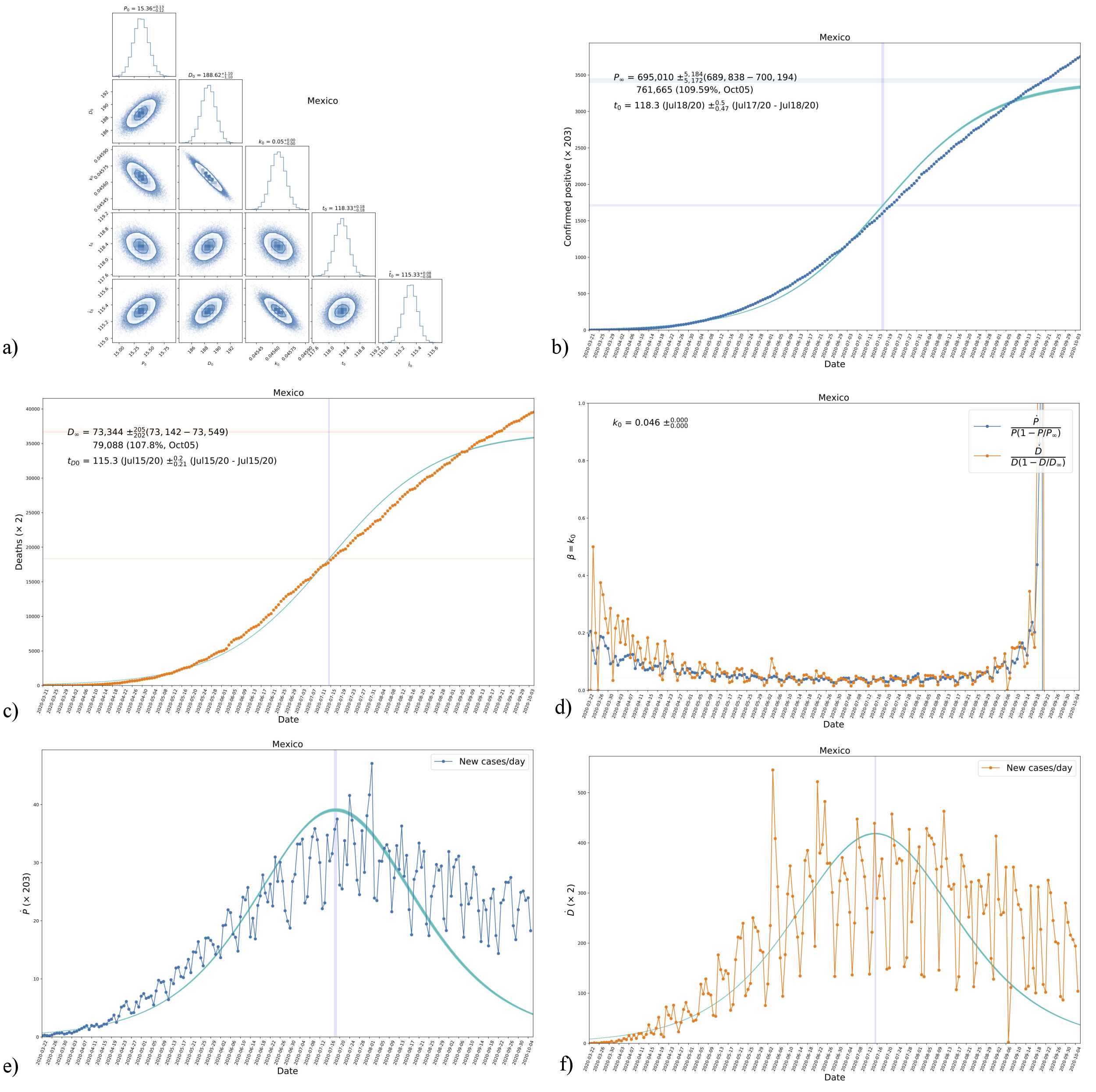
To fit the data, we will use the emcee code [25], a python code, to random sample a probability distribution that has been extensively used for a variety of applications. See Appendix D for a wider explanation of how the likelihood for this model was prepared (as well as for the others presented in this work). For the analysis, a set of 100 chains with 30000 steps in each one were run. The results are shown in Fig. 2 for the free parameters of our model. A common feature of all the countries we considered, not just the one shown in Fig. 2, is that the values of P
i
, D
i
, t
0, k
0, k
1, u
0, and
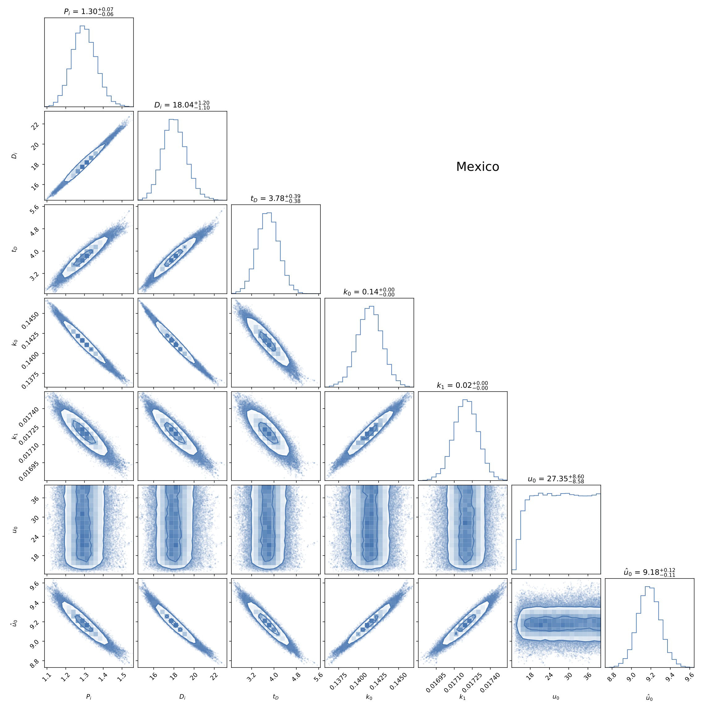
FIGURE 2 Triangle plot of the fitting to data from Mexico (see also Fig. 1) of the parameters P
i
, D
i
, t
D
, , k
0, k
1, u
0, and
We have applied our model to the data of 9 other countries, which at the moment of writing are the countries with the highest number in cumulative positives and deaths in terms of their population size, and the fitting results are summarized in Table I. As said before, P ∞ and D ∞ are the expected final numbers for the cumulative positives and deaths in each case, even for countries that have not yet reached an asymptotic value.
TABLE I Fitted values of parameters in model A, see Eqs. (18), as obtained from the data of different countries. The confidence regions for the parameters in the case of Mexico are shown in Fig. 2.
| Country |
|
|
|
|
|
|
|
|---|---|---|---|---|---|---|---|
| Mexico |
|
|
|
|
|
|
|
| Peru |
|
|
|
|
|
|
|
| Belgium |
|
|
|
|
|
|
|
| Bolivia |
|
|
|
|
|
|
|
| Brazil |
|
|
|
|
|
|
|
| Chile |
|
|
|
|
|
|
|
| Ecuador |
|
|
|
|
|
|
|
| United States |
|
|
|
|
|
|
|
| United Kingdom |
|
|
|
|
|
|
|
The delay time between positives and deaths, t D , is for all cases lower than 20 days, which is consistent with the general fact that all deaths were first confirmed as positive, and then t D will represent the delay time between a positive test and the occurrence of death.
Next are the parameters of the transmission rate β, where we note a strong similarity in the values of the different countries. First, we recall that β(0) = k
0, and then this parameter is the value of the transmission rate at the start of the time series. Likewise, parameter k
1 is the decay rate of the transmission rate. The last two columns in Table I show the values of the integration constants u
0 and
Other quantities of interest, which are derived from the basic parameters in Table I, are also shown in Table II. The first one is the total
population number N, which within model A is understood to be
the total population in susceptible form for the spreading of the disease. We
can see that this number is less than the total population in the case of
countries that seem to have the epidemics under control, but in some others, it
can be much larger than the whole world population. This only signals the lack
of convergence of model A for the parameters u
0 and
TABLE II Fitted values of extra parameters in the case of model A, for the same countries as in Table I. Shown are the total population number N, the half-life time t 1/2 of the transmission rate β, see Eq. (13b), the crossing times of half the asymptotic values of cumulative positives and deaths, t 50 and t D50, respectively, see Eqs. (15), in number of days after the start of the time series.
| Country |
|
|
|
|
|---|---|---|---|---|
| Mexico |
|
|
|
|
| Peru |
|
|
|
|
| Belgium |
|
|
|
|
| Bolivia |
|
|
|
|
| Brazil |
|
|
|
|
| Chile |
|
|
|
|
| Ecuador |
|
|
|
|
| United States |
|
|
|
|
| United Kingdom |
|
|
|
|
More meaningful is the half-lifetime of the transmission rate represented by t 1 /2, which is directly calculated from parameter k 1. The lowest value corresponds to Belgium, with the disease decreasing by half every 15.09 days, whereas the highest corresponds to Chile, for which the disease decreases by half every 115.51 days. It is interesting to note the relation between t 1 /2 and the measures taken to control the epidemics, as the lower values are for countries with the strictest lockdown measurements.
Almost as meaningful as t 1 /2 are the values of the halfcrossing times t 50 and t D 50, calculated from Eq. (15b). The lowest values correspond to Belgium, for which the halfcrossing occurred just 38 and 35 days after the report of the first deaths. The largest values are for Brazil, resulting in 157 and 124 days, respectively.
In the top and middle panels of Fig. 3, we show the comparison of data with the estimated evolution curves from our fitting, where the latter are represented by 500 instances of the model using a sample of values around those of maximum likelihood. In general we see a better a very good agreement with the data, which suggests that Eqs. (18) represent well the evolution of real data. For reference in the plots, we also show the times at half-crossing, around which the number of confirmed positives and deaths were half the asymptotic values P ∞ and D ∞, respectively.
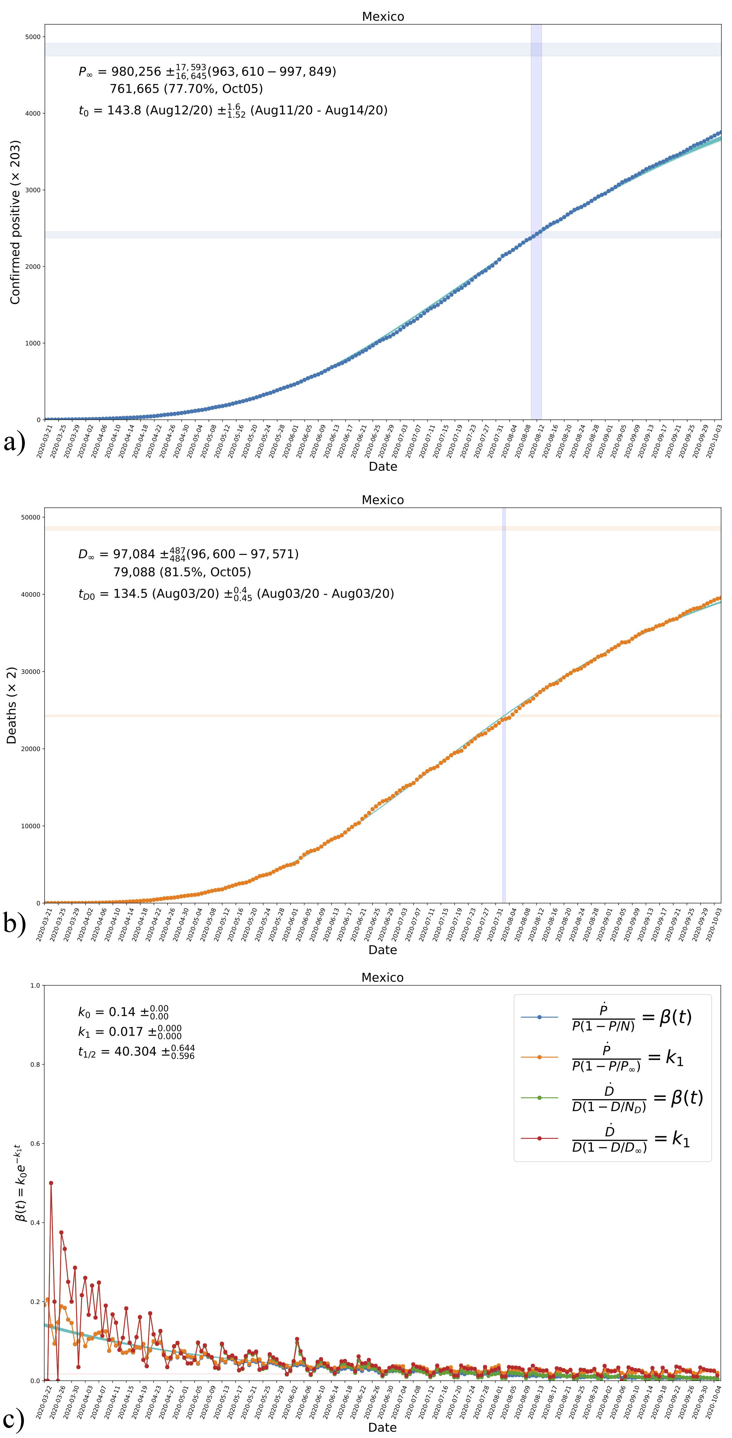
FIGURE 3 The resultant evolution curves of accumulated confirmed positives a) and deaths b) in the case of Mexico, according to the values in the triangle plot in Fig. 2. Shown in the figures are the obtained asymptotic values P ∞ and D ∞, see Eq. (7) and Table I, in the top blue-shaded horizontal regions. The vertical blueshaded regions mark the time of half-crossing in each case; the region for I ∞ /2 is also shown for reference. c) The resultant evolution of the transmission rate β according to the parametrization in Eq. (13a) and its comparison with data, see Fig. 1 and Tables I and II. Shown are also the obtained values of the parameters k 0 and k 1 and the corresponding half-life time of the disease t 1/2 . The horizontal red-shaded region represents the obtained value of k 1, see Eq. (12b). See the text for more details.
Also, in the bottom panel of Fig. 3, we show the time evolution of the transmission rate β(t) and its comparison with data, represented here by the new daily cases of both confirmed positives and deaths. We see a very good agreement with the combination of data that, in principle, represents the transmission rate. Likewise, there is good agreement with the combination that represents the parameter k 1, which in the plot is represented by the horizontal red-shaded region.
As an extra comparison with data, we show in Fig. 4 the derivative of both confirmed positives and deaths as obtained from the fitting to data and using the analytical formula (2) for each case. It must be recalled that the trend of new cases was not used for the fitting to data, and then the mentioned comparison is useful as an extra validation of the fitting, even if it does not appear to be as good as for the cumulative cases in Fig. 3. Additionally, the results show that the derivative of the model can follow the daily evolution of the disease and not just the global trend.
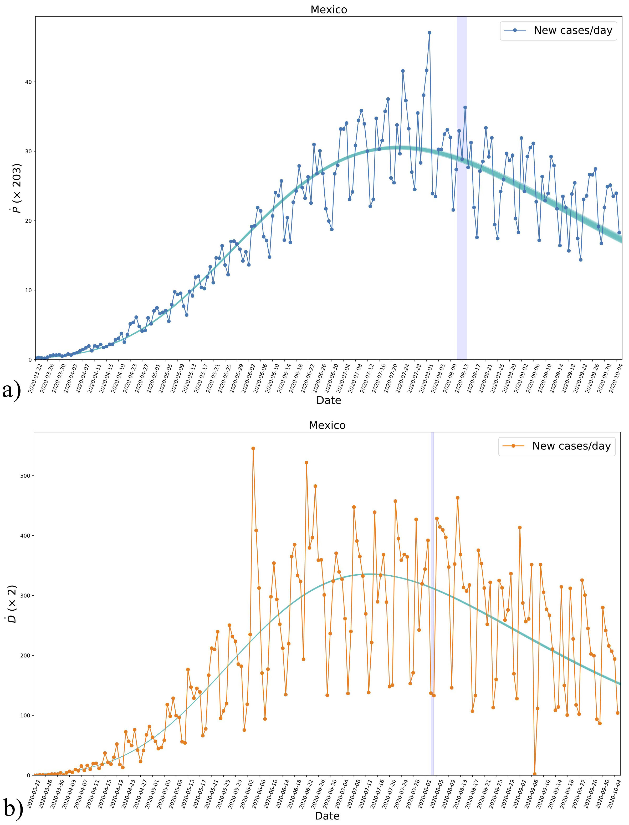
FIGURE 4 The derivatives Ṗ and Ḋ for positives a) and deaths b), respectively, obtained from the data of new daily cases and the analytical expression (2) using the parameters fitted to the data, see Fig. 2. Even though the new daily cases were not used for the fitting, we see a consistent agreement with the results. The blueshaded vertical regions mark the crossing of half the asymptotic values in each case as in Fig. 3. See the text for more details.
As the last feature, we show in Fig. 4 the time of halfcrossing with a vertical blue-shaded region, which indicates that the maximum of new daily cases is reached some days before and then the presence of such maximum seems to be a necessary condition for the inflection of the cumulative cases.
3.2. Model B and fitting to data
As explained before, for model B, we will consider the following parametrisation of confirmed positives and deaths, in cumulative numbers,
where the variable u has the same form as in Eq. (13b). For this parametrization, we obtain directly that P/P ˙= β and D/ Ḋ = βe k1tD , and also obtain the same limit results as in
Eqs. (14). Explicitly, the functional form of model B (19) is
which is no other but the Gompertz function [20,21,26]. In this way, one can see that there is a direct connection between the SI model and the Gompertz function, mediated by an exponentially decaying transmission rate and what we called the large-N limit.
As said before, for this simplified model, see Sec. 2.3 above, one can find analytical expressions for different quantities of interest, which are actually the same one obtains from the Gompertz function (20) [21]. The first ones are the asymptotic values at t → ∞, which are given by P ∞ = P i e k0/k1 and D ∞ = D i e k0/k1 , for confirmed positives and deaths, respectively.
Another analytical result is the time for the inflection of the curve, which we denote by t 0 following the nomenclature of the time-independent SI system. The expression is
where we have included the time shift t D of the function D(t). Likewise, the numbers of confirmed positives and deaths at the inflection time are
which is the same functional form for both of them. One can easily see that P 0 = P ∞ /e and D 0 = D ∞ /e.
The inflection point also corresponds to a maximum in the derivative of Eqs. (19), and then we find
This time the model has five free parameters: P i , D i , t D , k 0 and k 1, and as in model A the last two of them are common to both confirmed positives and deaths. We will again assume some level of intrinsic error by using a Poisson distribution and the same normalization of the data so that the first point is of order of an unity. Given this, we consider flat priors in the form: 0 < P i < 10, 0 < D i < 10, 0 < t D < 100 and 0 < k 0 , k 1 < 3.
We again took the emcee algorithm, see Appendix D, using 100 chains with 20,000 steps in each one. The results are shown in Fig. 5 for the free parameters of our model. As happened before in model A, the values of P 0, D 0, t 0, k 0, and k 1 are well constrained by the data, and their values are similar and of the same order of magnitude as those of model A. This is seen from a quick comparison of the common parameters in Figs. 2 and 5.

FIGURE 5 Triangle plot of the fitting to data from Mexico of the parameters P 0, D 0, t D , k 0, and k 1 of model B described in Sec. 3.2. In general, and similarly to model A in Fig. 2, all parameters are well constrained by the combination of cumulative confirmed positives and deaths. See the text for more details.
The fitting values of the parameters of model B for the same countries as in model A, are shown in Table III. Firstly, we notice again that the asymptotic values P ∞ and D ∞ are quite similar to those obtained for model A . This indicates that model B, although simpler than model A, is also a good model to follow the evolution of the cumulative cases. Secondly, the similarity in the results extends to the other common parameters between the models, as is the case of t D , k 0, and k 1, which again supports the validity of model B to fit the data under simpler assumptions.
TABLE III Fitted values of parameters in model B, see Eqs. (19), as obtained from the data of different countries. The confidence regions for the parameters in the case of Mexico are shown in Fig. 5.
| Country |
|
|
|
|
|
|---|---|---|---|---|---|
| Mexico |
|
|
|
|
|
| Peru |
|
|
|
|
|
| Belgium |
|
|
|
|
|
| Bolivia |
|
|
|
|
|
| Brazil |
|
|
|
|
|
| Chile |
|
|
|
|
|
| Ecuador |
|
|
|
|
|
| United States |
|
|
|
|
|
| United Kingdom |
|
|
|
|
|
The same happens when one compares the fitting results of the half-life time t 1 /2 with those in Table II; they are very similar to each other for the respective countries. The similarity extends for the case of the inflection times t 0 and t D 0, which are lower than the half-crossing times of model A. This is as expected, given that in model A, the half-crossing should happen after the inflection of the resultant evolution curve. As in Table II, we find that the lowest characteristic times correspond to Belgium, whereas the highest correspond to Bolivia.
We repeated the comparisons between the data and model B in the same form as in Fig. 3. The new results are shown in Fig. 6. As anticipated in Sec. 2.4, model B is also good at following the trend of the data and the only changes are in values of the fitted parameters, which also result in changes of the final quantities P ∞ and D ∞, although the obtained values are consistent one to each other in their order of magnitude in the two models.
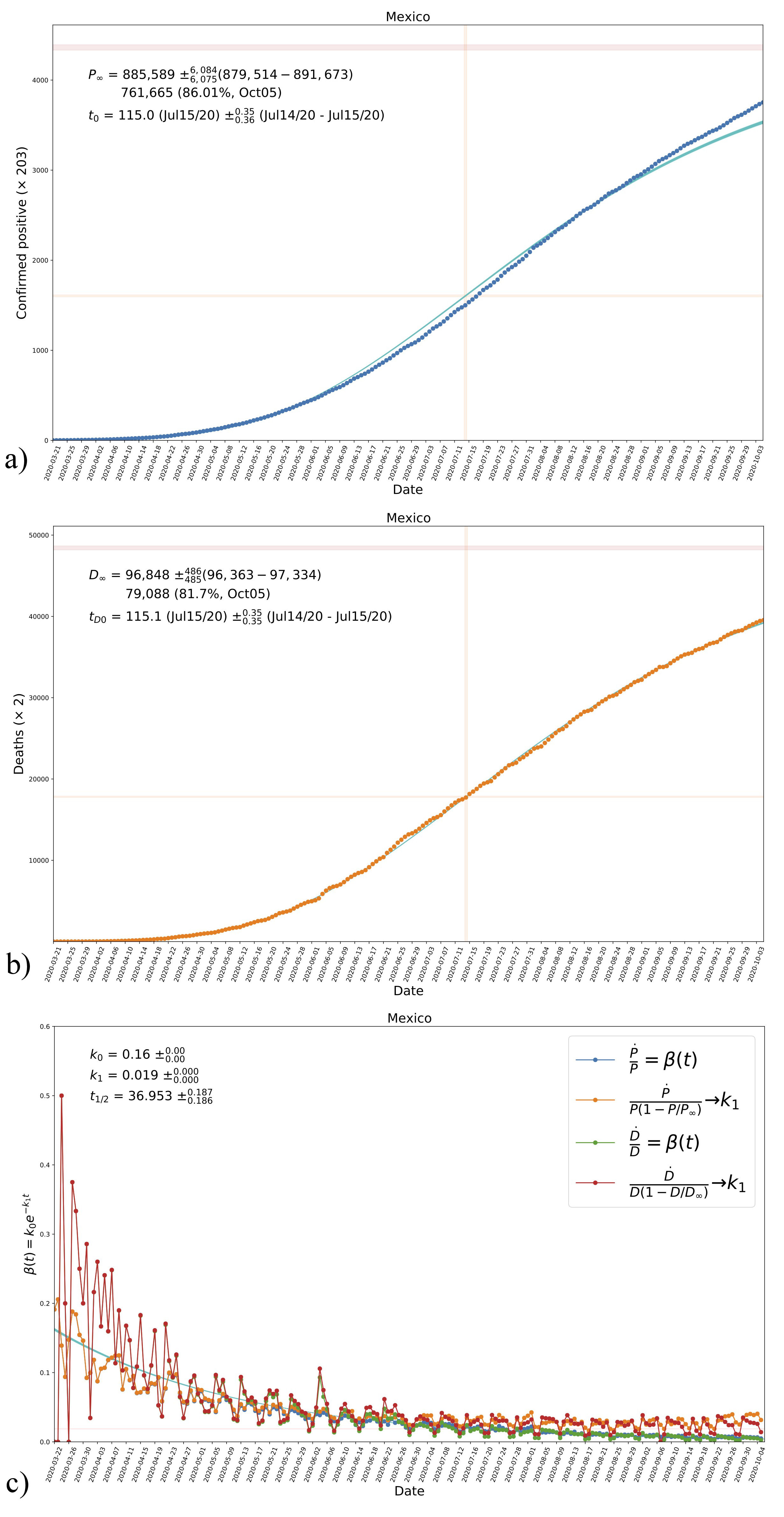
FIGURE 6 The resultant evolution curves of cumulative confirmed positives a) and deaths b) for model B in the case of Mexico, according to the values in the triangle plot in Fig. 5. Shown in the figures are the obtained asymptotic values P ∞ and D ∞, see Eq. (7) and Table IV, in the top blue-shaded horizontal regions in each plot. The vertical blue-shaded regions mark the time inflection in each case; the region for P(t 0) is also shown for reference. c) The resultant evolution of the transmission rate β according to the parametrization in Eq. (13a) and its comparison with data, see Fig. 1 and Tables III and IV. Shown are also the obtained values of the parameters k 0 and k 1 and the corresponding half-life time of the disease t 1/2 . The horizontal red-shaded region represents the obtained value of k 1 see Eq. (12b). See the text for more details.
TABLE IV Fitted values of extra parameters in the case of model B, for the same countries as in Table I. Shown are the half-life time t 1/2 of the transmission rate β, see Eq. (13b), and the inflection times of cumulative positives and deaths, t 0 and t D0, respectively, see Eqs. (21a).
| Country |
|
|
|
|
|---|---|---|---|---|
| Mexico |
|
|
|
|
| Peru |
|
|
|
|
| Belgium |
|
|
|
|
| Bolivia |
|
|
|
|
| Brazil |
|
|
|
|
| Chile |
|
|
|
|
| Ecuador |
|
|
|
|
| United States |
|
|
|
|
| United Kingdom |
|
|
|
Finally, in Fig. 7, we show the comparison of the derivatives of model B for both the confirmed positives and deaths with their corresponding data. We also see a good agreement in both the time profile and the location and height of the maximum points in the two plots. This time model B is more easily manageable, and we show the maximum daily new cases as expected from the theoretical expectations. Notice that the time at the location of the maximum is the same as that of the inflection time t 0 in the evolution of the cumulative cases, see Fig. 6.

FIGURE 7 The derivatives Ṗ and Ḋ for positives a) and deaths b), respectively, obtained from the data of new daily cases and the analytical expression of model B, see Eq. (19), with the parameters fitted to the data, see Fig. 5. Even though the new daily cases were not used for the fitting, we see a consistent agreement with the results. The blue-shaded vertical regions mark the inflection time in each case, as in Fig. 6, whereas the blue-shaded horizontal regions mark the maximum values of each case. See the text for more details.
4. Final comments
We have presented a generalization of the well-known SI system to include the possibility of a time-dependent transmission rate and used a particular exponential-like parametrization of it to fit and describe the evolution of real data for the epidemics of Covid-19.
Although the use of time-dependent transmission rates is not new in the literature of epidemic models, this is the first time that such an approach have been applied to the SI system, for which there exists an analytical form of the general solution. The latter is the standard logistic function, but now with a generalized time variable that results from the direct integration of the transmission rate. These features simplify the handling of the model and ease its comparison with data.
For the functional form of the time-dependent transmission rate, we chose a decaying exponential with two free parameters, the first one for the initial value of the transmission rate and the second one for its decay rate. In this form, our generalized model has enough complexity to fit the data reliably, whereas at the same time provides meaningful quantities to describe the evolution of cumulative positives and deaths.
One of those meaningful quantities is the decay rate, and the related one is the half-life time of the transmission rate. It was clear from our results that the half-life time is shorter for countries that have taken the strictest measures of public containment. Other countries seem to have an almost three times larger half-life time, which means that it will take longer for them to tame the epidemics. Even though in medical terms one may wish to have slow epidemics to avoid saturation of hospital services, this also means that containment measures will have to take place for longer too, which may result in a general public being tired of the governmental intervention.
Our model also suggests an interesting correlation between the initial value of the transmission rate and its decay rate: countries that experienced faster dissemination at the beginning are the ones that report a larger decay rate, as is the case of Belgium and the United Kingdom. Likewise, countries with a slow initial spreading seem to be the ones with also a lower decay rate. These last countries were not hit as badly as others at the start of their epidemics, but all so far indicates, according to our models, that they will have some of the highest death tolls in the world.
A surprising result was the connection of the SI system with the Gompertz function. As explained in the text, such connection requires some assumptions in between, mainly that the transmission rate is time-dependent with an exponential form, and that we consider a largely susceptible population. Although the Gompertz function is quite useful for a plethora of growth phenomena, ours is the first study that shows a derivation of it from an infectious model.
One final note on the fittings we obtained for the models. The Bayesian inference is an appropriate method to fit data if one faces a unique realization of the natural phenomenon under study, which is the case of the present epidemics of Covid-19, as the data reported by each country is not at all the result of repeated experiments under controlled conditions. In this respect, the Bayesian analysis allows us to do a sampling of values of the free parameters around the point of maximum likelihood. This does not mean that one finds the best and only fitting to data, but the best possible fit given the proposed model. This helps to explain the well-defined confidence regions in the triangle plots of the fitted parameters, even though the resultant curves may not even look good by eye when compared to data (see, for instance, model C in Appendix C).
The numbers reported here are not definitive, and they may change considerably if the epidemics follow a different evolution soon. However, we believe that our models may help characterize the present evolution of the disease and can be considered to decide about further public measures to handle the epidemics.