


 nova página do texto(beta)
 Inglês (pdf)
 Artigo em XML
 Referências do artigo
 Enviar este artigo por email
 Citado por SciELO
  Similares em
SciELO
Similares em
SciELO 
 Permalink
1. Introduction
William O. Kermack and Anderson G. McKendrick described the SIR model for the first time in 1927 [1], which was the pioneering model for the study of epidemics using differential equations. There was knowledge regarding the behavior of disease epidemics in those years, and it led to the proposal of a mathematical model which could describe the evolution of arbitrary infections during an epidemic. Kermack and McKendrick proposed a classification of individuals in a population N, susceptible S, infected I, and recovered R.i The set of individuals should then behave accordingly with the following system of equations in a certain time period
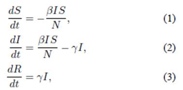
where S(t),I(t),R(t) describe the number of susceptible, infected, and recovered individuals as a function of time, respectively. The recovery and transmission rates are given by λ and β, respectively. The system of non-linear differential (1-3) has been solved algebraically [2] (see Fig. 1), and analytically [3].

FIGURE 1 Algebraic solution to the system of differential (1-3), assuming non-vital dynamics, where N = 1, S(t)+I(t)+R(t) = 1, with β/γ = 2, I(0) = 10−3, S(0) = 1− I(0).
Kermack and McKendrick used their model to analyze the data from the 1906 bubonic plague of Bombay and obtained a great quantitative approximation that matched the number of deaths caused by the Yersinia pestis bacterium. The SIR model was used to study the dengue fever breakouts, caused by mosquito bites, of 1997 in Cuba and 2005 in Venezuela [4]. The model was also used to analyze the 1997 outbreak of classical swine fever in the Netherlands, which is a highly contagious viral disease that affects herds of pigs and wild boars [5].
In December 2019, a new coronavirus (CoV) was detected owing to a harsh pneumonia outbreak that is believed to have originated in a wet market of Wuhan, China. Later in January 10, 2020, the first genome sequence was made publicly available, revealing a similarity with already known forms of coronaviruses such as the MERS-CoV and more closely to the SARS-CoV. The novel coronavirus was designated severe acute respiratory syndrome coronavirus 2 (SARS-CoV-2) by the Coronavirus Study Group of the International Committee on Taxonomy of Viruses [6]. As of January 20, 2021, according the statistics from the World Health Organization (WHO) [7], there are a total of 94,124,612 confirmed cases and 2,034,527 confirmed deaths due to the SARS-CoV-2.
Scientists from all over the world rushed immediately to find an effective antiviral treatment against the SARS-CoV-2, which is the responsible agent for the ongoing coronavirus disease (COVID-19). The Oxford-AstraZeneca collaboration was the first to publish results from phase III clinical trials of a COVID-19 vaccine on December 8, 2020 [8]. On December 11, 2020, the U. S. Food and Drug Administration (FDA) issued the first emergency use authorization (EUA) for the Pfizer-BioNTech COVID-19 vaccine, and followed with a second EUA for the Moderna COVID-19 vaccine, allowing them to be administered to the public [9, 10]. Mexico’s FDA analogue Comision Federal para la Protección contra Riesgos Sanitarios (COFEPRIS) also issued an equivalent emergency use authorization on December 11, 2020, for the Pfizer-BioNTech COVID-19 vaccine [11]. On January 4, 2021, the COFEPRIS issued a second emergency use authorization for the AstraZeneca COVID-19 vaccine [12], allowing both companies to distribute their vaccine in the country for their application to the public. Real-time updates and information on the disease and the vaccines can be found summarized in [13]. The collective efforts consist of developing more vaccines, social distancing protocols, and officially imposed quarantines. Additionally, a series of mathematical models have been implemented to estimate the scope and transmission capacity, taking into account numerous factors, of the COVID-19, among them the SIR model [14].
2. Computational model
The computational model of this work implements colliding particles that move freely inside a square domain which is never abandoned by the particles. The viral transmission rules which the particles obey are based on the person-toperson spread mechanism, that is, direct and indirect contact as sneezing, coughing, and touching contaminated surfaces.
2.1. Number of particles, N, and the collision detection method
A determined number N of particles i with a
specific mass are allocated inside a square domain of area Ω =
l
x
×l
y
. The intrinsic RANDOMNUMBER subroutine from Fortran 90 is called to
assign each particle a random position
The numerical time integration for the position and velocity of the particles was tested using the Adam-Bashforth, Runge-Kutta, Euler, and Verlet methods. The Verlet method of order O(∆t 4) was ultimately selected owing to its high accuracy and low computational cost, and was developed on a prediction-correction algorithm [15] described as
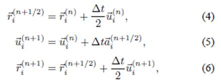
where the superscript n represents the time which is being
calculated. The time step ∆t = 1 × 10⁻⁴ s is a
constant, and
where

In Eq. (7), the sum is performed over all neighboring
particlesj, m
i
= 1 kg for all i particles, κ = 50 N/m
is the spring constant,
2.2. Particle classification and transmission rules
In a broad manner, the Kermack-McKendrick model explains mathematically how a epidemic disease spreads amongst a determined number of individuals of a population with certain characteristics, and how its effects come to an end after a time period. In this work, the characteristics of the individuals are narrowed to susceptible S, infected I, and recovered R. Demographic events such as deaths, births, immigration and emigration are not considered.
In our model, each case begins with all particles classified as susceptible, except for one randomly infected particle I z (patient zero) with the capacity to alter the state of every particle it encounters. Naturally, every new infected particle now has the capacity to also infect susceptible particles. In order to yield results that can resemble a real-life scenario with more accuracy, the at-contact infection mechanism is replaced by an infection mechanism based on a probability parameter p c and is implemented as follows. All infected particles will be surrounded by an infection radius R c = 0.03 m with a known p c , when a susceptible particle approaches an infected one close enough to be inside R c , a randomly assigned value is given to a variable rnd. If rnd > p c the state of the susceptible particle remains unchanged, giving it the possibility of not becoming infected even if it still inside R c . On the other hand, if rnd ≤ p c the susceptible particle now becomes infected. This procedure is only assigned once to susceptible particles every time they are inside R c . An infected particle changes its state to recovered after exceeding a recovery time t r = 25 s (infectious period), and a recovered particle cannot become infected again. The recovery time has been considered a constant for all infected particles. In this work the value for t r is irrelevant, although it is subject to further discussion.
3. Results
3.1. Free-for-all scenario
The initial configuration, referred to as free-for-all scenario, consists of particles created inside a square domain of sides Ω = 1 × 1 m, with random position, moving in random directions with a constant velocity magnitude of U = 0.05 m/s, colliding into each other with a p c = 0.4 (which remained constant for all configurations). In this scenario, the initial conditions are S(0) = 199 and I(0) = 1. The evolution of the position of all particles is depicted in Fig. 2, where the first 9 time frames were captured every 6.65 s for a maximum time, t max, of 120 s. When an infected particle changes the state of a susceptible particle to infected, the latter can change the state of other susceptible particles while it remains within the recovery time, consequently generating an exponential change of susceptible to infected particles (see Fig. 3a)). The maximum number of infected particles, I max, was recorded at t = 32.3 s for I max = 186, representing 93% of the total population. Following I max, an exponential decay of infected particles is recorded along with an increase in the number of recovered particles. Eventually, the entire population shifted from susceptible to infected, and finally all recovered at the end of the simulation.

FIGURE 2 All susceptible particles (•) move freely. At t = 0.0 an infected particle (∗) is introduced and begins the infection process, i.e., the start of the pandemic. An exponential growth is observed at t = 6.65 s and t = 19.95 s. At t = 26.60 s the first recovered particles (◦) are observed. Later, an exponential decay of infected particles occurs at t = 33.25 and t = 29.90 s. Finally, the number of recovered particles is predominant.
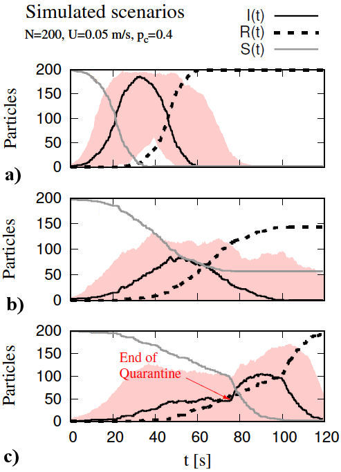
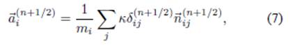
FIGURE 3 Projection curves where susceptibles are solid gray line, infected are solid black line, and recovered are dashed black line. a) free-for-all, b) quarantine, and c) end-of-quarantine. The number of infected particles for each scenario is inside the red background region, which is the result of 400 additional simulations. In all cases, the ordinate shows the number of particles, whereas the abscissa represents time.
3.2. Quarantine scenario
The second configuration, referred to as quarantine, begins by randomly distributing the particles inside the domain and fixing 80% of the particles as immovable regardless of collisions and changes of state. The remaining 20% of particles have the same constant velocity U = 0.05 m/s and move in random directions with I z included in this percentage. The stationary particles can change the direction of moving particles when they interact, and they can also become infected (see Fig. 3b)). A similar behavior to that of the free-forall scenario was observed, that is, an exponentially growing number of infections which eventually decays. The maximum number of infected particles, I max, was recorded at t = 47.3 s for I max = 85, representing 42.5% of the total population. At the end of the simulation, a total of 143 particles shifted from infected to recovered, representing 71.5% of the population; whereas 57 particles kept their initial susceptible state, representing 28.5% of the population.
3.3. End-of-quarantine scenario
The third configuration is referred to as end-of-quarantine owing to its inherited configuration from the quarantine scenario. This configuration begins identical to the quarantine scenario, until a t 0 = 75 s is reached, and at this point, all particles are free to move, recovering the free-for-all scenario. Prior to t 0, a very similar behavior to the quarantine scenario was observed. After t 0, a new exponential growth of infected cases was recorded (see Fig. 3c)). The maximum number of infected particles I max was recorded at t = 89.9 s for I max = 105, representing 52.5% of the total population. At the end of the simulation, a total of 193 particles shifted from infected to recovered, representing 96.5% of the population; whereas only 2 particles kept their initial susceptible state and 5 particles remained infected [4].
Every scenario was simulated 400 times with different seeds, i.e., the function RANDOMSEED was used for each new case while maintaining the parameters used for the previous scenarios as constant. For each scenario, Fig. 3 shows in red, the region where the results were obtained for the number of particles (I) according to the 400 simulated cases. In the free-for-all scenario (Fig. 3a)), we obtained a maximum from the set of all maxima belonging to each case of infected particles (I) as (I max)max = 197 representing 98.5% of all particles. In the quarantine scenario (Fig. 3b), (I max)max = 131, representing 65.5% of the total. Finally, in the end-of-quarantine scenario, (Fig. 3c), (I max)max = 171 which represents 85.5% of the total.
3.4. Transmission rate β, recovery rate γ, and basic reproduction number R 0
An analysis was performed on the recovery rate γ, the transmission rate β, and the basic reproduction number R 0 for all three scenarios. Initially, we studied the area under the curve for the set of data describing the number of particles (I), and the function that is obtained by multiplying the data of (I) by (S), these are A(I) and A(IS), where A represent the area under the curve computed using Simpson’s 1/3 method of numerical integration
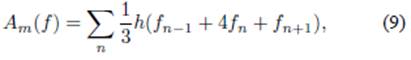
where h = 500∆t, and n = 1,3,5,7... is the index representing the data values contained in all simulated cases m = 1,2,...,400. Afterwards, Eqs. (1) and (3) from the Kermack-McKendrick model were used to study the behavior of the rates described by epidemiology, which, in their integral form, constitute the following identities

where all cases m considered the full set of data from a time t = 0 to t = t max. In our model, the recovery rate γ m represents the amount of new particles (R) over a unit of time over the number of susceptible particles within the population (see 4a)). The recovery rate β m is the ratio of particle-particle contact multiplied by the probability parameter p c (see Fig. 4b)). The basic reproductive number (R 0) m = β m /γ m is defined as the number of new infected particles within the infectious period of any arbitrary infected particleii (see Fig. 4c)).

3.5. Basic reproductive number R 0 as a function of particle density
The behavior of the basic reproductive number R 0 was analyzed as a function of the particles N (see Fig. 5). The domain size Ω was maintained constant with 1×1 m in order to achieve a proportional particle density ρ p = N/Ω to the total number of particles. It was noticed that R 0 increases monotonically for the free-for-all and quarantine scenarios. In the latter and former scenarios, the mean free path is shortened due to the high particle density, consequently increasing the ratio of particle-particle contacts as well as the transmission rate, thus validating the relation R 0 ∝ β. Regarding endof-quarantine scenario for time t = 75 s, a non-monotic behavior is observed, as can be seen from the inflection point at N = 178. For all cases, R 0 > 1, except for the quarantine scenario, at N = 75, R 0 = 0.8217. It is important to highlight that R 0 for end-of-quarantine scenario is very similar to quarantine scenario for particle densities greater than 250/m2.

4. Conclusions
In Fig. 3a), a monotonically decreasing function
is represented, where the number of susceptible particles declines with respect to
time, therefore, its change in time is negative, S
0(t) < 0. In turn, the number of
recovered particles increases with respect to time, i.e., it is
represented by a monotonically increasing function, making its change in time
positive, R
0(t) > 0. On the other hand, the
number of infected particles is non-monotonous and resembles a gaussian
distribution, having only one increasing region and one decreasing region. Besides,
the inverse of the recovery rate, described by (11), is in qualitative agreement
with the recovery time t
r
= 25 s. This can be seen in Fig. 4a),
where the free-for-all histogram shows that all cases reported a recovery rate close
to γ
m
= 0.04, making 1/γ
m
= 25. These results are in qualitative agreement with the description from
the Kermack-McKendrick model (Fig. 1). The
characteristic monotonic behavior of the curves in the quarantine scenario seems to
be conserved, showing certain similitude with the Kermack-McKendrick model, however,
limiting the movement of a great number of particles greatly affects the ratio of
particle-particle contacts, which consequently influences the transmission rate and
the basic reproductive number, respectively (see Figs.
4b) and 4c), where the arithmetic mean of the distribution of the
quarantine scenario,
Unlike the differential equation model, our model is able to modify the behavior of
the particles to simulate ending a quarantine before the number of particles
(I) reaches zero. This was hypothesized in order to study the
effects of relaxing social distancing measures just before planned. Prior to
t = 75 s, the results are similar to the quarantine scenario,
after the number of particles (I) varies, we observe for most cases
two infection stages corresponding to two maxima in the number of particles
(I). In some cases, the second growth stage is significantly
larger than the first one, reaching a maximum of 171 particles (I)
(85.5 %). As shown in Fig. 4c) the mean value
of the basic reproductive number distribution
In countries whose population density is relatively low such as New Zealand and Australia, the basic reproductive number R 0 of infectious diseases can be small when compared to that of countries with high population density such as Mexico, U.S.A, and China (refer to Fig. 5). This can be better understood by looking at the number of confirmed cases and deaths from COVID-19 as of October 16, 2020, for New Zealand and China [20,21].
Our particle model is a perfect disease transport model, contrary to local transmission models such as the cellular automata in [22]. Nevertheless, the qualitative results, presented in the latter and the current work, regarding the transmission rate, are very similar under a perfect mixing scenario such as the free-for-all. This is justifiable due to the strong relation between the transmission rate, the particle-particle contact rate, and the infective probability, which in the cellular automata model, the cell-cell contact ratio is constant, in turn only modifying the infective probability parameter. On the other hand, our model allows us to keep the probability parameter as a constant, while being able to modify the particle-particle contact ratio when the particle density is increased or decreased.
5. Discussion, observations, and notes to the reader
If the contact radius d is larger than the infection radius R c for all particles, then the infection rule is not satisfied and it is not possible to observe an overall evolution of the system. That is, the infected particle I z cannot change the state of susceptible (S) particles to infected (I), (see Sec. 2.2). This scenario is a perfect analogy to that of physical distancing in real life. A numerical implementation of a randomized contact radius could very well replicate a real life physical distancing behavior.
In epidemiological theory, the infectious period of an infected individual lasts until recovery or death (recovery time t r ), which is not the same for all individuals, however, for the sake of simplicity, we take the average t r of a certain population.
The infection radius R c estimates the radial distance at which an infected individual (I) can emit particles with pathogens by sneezing or coughing, which are, at some point, indirectly ingested or inhaled by a susceptible individual (S). This phenomenon was reported as one the main transmission modes of infectious diseases such as the common flu, SARS-CoV or SARSCoV-2 [23].
The probability parameter p c is related to the hygienic actions of a susceptible individual, such as hand washing [24], or the use of sanitary personal protective equipment (PPE) like face masks or gloves [25]. In principle, this parameter is unique of each individual in a population.
Obtaining real results implies great computational complexity, such as increasing the number of particles N to thousands (∼ O(103)) or millions (∼ O(106)), which represents larger computation times. This would also require simulations that resemble the behavior of real-life individuals in a social environment, and not as free particles.
A study on the effect of population density in infectious disease models [26] reveals that, for extremely dense populations, the saturation of individuals limits their ability to make come in contact with each other, thus decreasing the infection rate. We consider that our results do not contemplate particle saturation until N = 400 given that R 0 is proportional to β.

