


 nueva página del texto (beta)
 Inglés (pdf)
 Artículo en XML
 Referencias del artículo
 Enviar artículo por email
 Citado por SciELO
  Similares en
SciELO
Similares en
SciELO 
 Permalink
1. Introduction
The distribution of liquid steel in the mold affects the liquid steel free surface fluctuations and, therefore, the homogeneity of the cooling process of the slab. So, to improve the steel quality, it is necessary to visualize and measure the hydrodynamic liquid steel behavior inside the mold and inside the nozzle. However, the study of the phenomena related to the continuous casting process presents difficulties regarding its operational conditions. Liquid steel fluid dynamics present some disadvantages considering the elevated temperature at 1,873 K inside the tundish [1,2].
As a consequence of the above behavior, the visualization of the process is performed in experimental facilities using water as the working fluid similarity criterion to obtain a scaled model of the system [3]. It is a frequent practice to reproduce the fluid dynamics within the mold using a scaled, physical model because of the reduced geometrical dimensions of the system and ambient temperature to prevent hazardous conditions during the process [4-13].
Three-dimensional, transient numerical simulations are used to complement the flow pattern observations and to study the fluid-structure interaction where the liquid steel passes. Other variable include the operating conditions, for example, the casting speed, which can be reproduced to understand the fluid dynamics phenomenon [5,8-11,13-17].
In the continuous casting process, the Submerged Entry Nozzle (SEN) is used to transfer liquid steel from the tundish to the mold, therefore, it determines the liquid steel flow pattern and finally affects the heat transfer process [11,15-18]. A good SEN design is necessary to improve the quality of steel. In literature, various SEN models have been proposed to satisfy the demand for high-quality steel. For example, based on thin slab technology, the angle of the SEN exit ports could also be directed upward to avoid fluctuations in the liquidfree surface [7,19]. Additionally, a larger number of exit ports have been observed to improve the steel distribution to the mold [7]. The external geometry of the SEN has changed compared to the standard model to increase the casting speed of the slab [20]. The form of the exit flow was changed with different shapes in the exit ports to eliminate the vortices on the SEN flow pattern [12,18,21-23]. These are only some modifications to the standard shape of the SEN. Proper visualization and measurement tools need to be implemented to differentiate the flow regimes between the modifications of the internal walls of the nozzles and within the mold as well.
Concerning the approach of design modifications of external SEN geometry that could achieve a quasi-stable flow condition, they are based on design parameters which allow a constant flow during castings to be achieved. The SEN received a considerable drag force from liquid steel; however, it is possible to obtain the necessary conditions within the SEN volume and therefore on the liquid surface of the mold [24,25]. With the second approach based on the SEN design, significant energy savings can also be achieved in the process.
The performance of SEN can be evaluated by observations of the exit flow, as well as the flow inside the visualization cell. Numerous authors have applied experimental techniques to observe the flow at the exit ports and have used translucent materials to visualize the flow pattern inside the mold [9,12,13]. Other authors proposed numerical algorithms to evaluate the flow behavior within the SEN [5,10,11,15,24,26]. However, to the authors’ knowledge, there are no published works devoted to the SEN internal flow pattern measurements.
In the present work, the geometrical, kinematic, and dynamic similarity criteria have been used to scale the physical model of the SEN [3]. The main aim of the experiment is to reproduce and analyze the hydrodynamics within the nozzle and the way it affects the exit of the flow by the ports.
2. System description
The experimental installation consists of two systems, the first one is called a “visualization cell” and is a rectangular prism, made of translucent acrylic with a thickness of 0.009 meters. The square base has 0.135 meters on the side and a height of 0.200 meters. The lateral walls have rectangular, transparent solids called “aligners” that locate the nozzle to the rectangular volume as seen in Figs. 1 and 2.


The nozzle is a 1:1/3 scaled model of a conventional SEN for the continuous casting process of a standard slab. It consists of two elements, the first one is made of orthophthalic unsaturated polyester resin to obtain the translucent properties required to observe the internal flow. The resin is a thermoset and must be cured from the liquid state to the solid state. This material was chosen based on its transparent properties after the curing process, ease of molding, machining, and low production costs. Previously, a wooden mold was built and the liquid resin with catalyst was poured into the mold. The catalyst does not take part in the chemical reaction, but merely activates the solidification process. After the resin is clear, the inlet port and the two exit ports can be machined. The second element was built in black polyoxymethylene, POM, to prevent reflections and is shown in Fig. 2. Because of the required displacement of this element, the bottom of the SEN is constructed as a different part to characterize the different operating conditions during the life of the nozzle.
The SEN model has one rounded inlet port of 0.0254 meters of internal diameter at the top and two rounded exit ports, 0.020 meters of internal diameter with a −15◦ angle of downward inclination, as shown in Fig. 2. The “pool” section has a bottom part at the base of the outlet ports.
A closed hydraulic circuit was designed to supply the water using a 1 H.P. centrifugal pump with a valve to control the flow rate of the liquid from a 100-liter tank located at the bottom of the experimental rig. The liquid flows into the system and is measured by a calibrated Dwyer VFC-153 flow meter, as shown in Fig. 1.
The nozzle discharges the water into the visualization cell, at the base wall the cell has an outlet bore of 0.00254 m in diameter to send back the water to the tank. The pump returns the water to the nozzle and the water recirculates it in a closed-circuit as shown in Fig. 2.
The second component of the experimental rig consists of an aluminum frame to position the cell in the visualization system, which is often used to align the cell with the camera. The camera was mounted on the base of a tripod that helped to align the camera with the visualization system as seen in Fig. 1.
3. Operation conditions. Experimental setup
During the tests, the operating conditions in the facility were recorded by a weather station in the Applied Hydraulics and Thermal Engineering Laboratory in Mexico City. The measurements were: relative humidity 56%, atmospheric pressure 78,000 Pa, and local temperature 294.15 K.
The visualization cell was reduced in size to achieve the minimum distance between the camera and the nozzle. The linear distance between the camera lens and the visualization cell is approximately 0.05 meters as shown in Fig. 3. The distance between the nozzle and the cell walls allows observation of the exit flow and prevents the camera lens from capturing the ‘flickering’ of the bubbles.
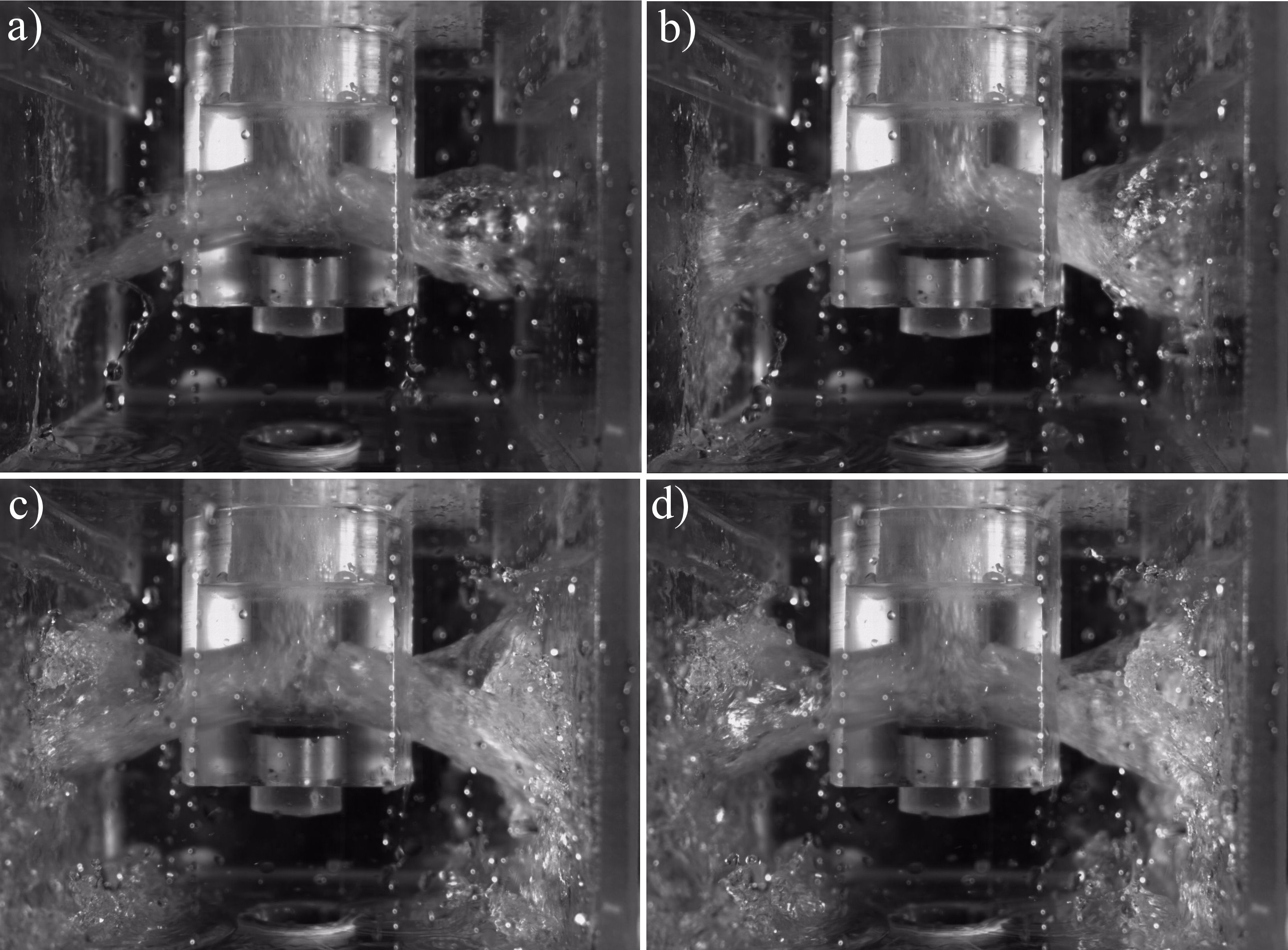
FIGURE 3 Images of the SEN flow inside the visualization cell at different times. a) 0.16 seconds, b) 0.2 seconds, c) 0.22 seconds, d) 0.26 seconds of the experiment beginning.
The centrifugal pump begins its operation and sends the water to the hydraulic circuit at a steady flow of 35 liters per minute. At the beginning of the test, we observed air bubbles in the system, even in the cell. The system worked for approximately 300 seconds to achieve quasi-stable conditions in the cell and after that time, there were not more bubbles in the system.
To illuminate the plane of visualization within the models, a LED light source model SLXLS-FL with 0.180 × 0.140×0.100 m dimensions, 20 W of electrical power, and 120◦ of light aperture was used. A DualPower 15-1000 laser source of 150 W was used to illuminate the plane and measure the flow characteristics in the PIV tests [27].
The water used in the PIV experiments was seeded with particle tracers of 10 µm diameter void glass spheres covered with silver.
The camera used in the visualization and PIV experiments was the Speedsense 9040, with a Nikon lens AF 2485/2.8-4D IF, which was configured to capture photographs of 1600×1200 pixels [28]. The total number of images in each experiment was 2000, the display refresh period was 0.100 s, and the time between frames was 0.00020 s, with a trigger rate of 500. These settings allowed us to record two seconds of the process.
4. Visualization cell
Visualization is the first step to qualitatively analyze experimental results; this step is important to understand the general fluid flow behavior in the cell. The distance between the light source and the wall of the cell was 0.5 meters at 45◦ to prevent the reflections on the camera.
When the system is in operation, the flow passes through the SEN and finally goes to the tank in a closed-circuit. Inside the SEN, the flow is split into two in the central lower zone of the SEN to both exit ports, and the flow from the SEN to the visualization cell.
Figure 3 shows the visualization cell and the transparent model of a nozzle, the two exit ports, and the pool region in the lower region of the cell at four separate times: (a) 0.16 seconds, (b) 0.2 seconds, (c) 0.22 seconds, (d) 0.26 seconds.
Figure 3a) shows how the flow exits the SEN at the first stage. While the system continues to work, Fig. 3b) shows when the left jet hits the sidewall of the visualization cell. It is also possible to observe that the left jet is larger than the right jet of the nozzle. Figure 3c) shows that both jets enter the cell visualization cell, while the lateral walls also splash the internal volume. Finally, Fig. 3d) shows another moment when the right jet is larger than the left jet.
Figure 3 shows in a sequence of four images, that there is a difference between the left and the right exit ports. The left port sends more fluid than the right exit port at one time and the swirl path between the exit ports is opposite, as shown in Figs. 3a) and 3b). 0.22 seconds into the experiments, the left exit port jet has a lower exit angle than the right exit port, Fig. 3c. The aperture angle of the jets on both exit ports are 47 and 53 degrees, these measurements are close enough. At 0.04 second, the flow conditions in both exit ports change significatively, Fig. 3d).
In the supplementary material section, a video of the experiment shows the left exit port, the upstream flow hits the upper wall of the port and continues to flow. Then, it hits the lower wall of the port, the flow begins to hit the walls of the port and forms a spiral flow structure. The right exit port has the same flow activity in the opposite direction; however, the mass flow between the exit ports is not the same.
In the same video, the size of the jets depends on the mass flow rate on each port. The jets fluctuate because of the interaction of the two internal vortexes found in the lower zone of the SEN, first reported by Real et al. in 2006 [17]. The vortices switch their size, as well as the location inside the SEN, and change the exit flow pattern of the visualization cell. The findings reported in 2006 can be assured and the results described in this work are consistent with the same geometrical characteristics and operational conditions.
Because of the high speed and high resolution of the camera, it is possible to observe the fluctuations in the size of the exit jets. The observed data help to explain how these variations are present in the fluid dynamics within the mold. It is also possible to obtain the frequency of variations of swirl directions of the exit jets and it will be compared in future work with the frequency of the free surface variations in the mold.
5. Analysis by particle image velocimetry
The PIV technique was used to measure the velocity field inside the SEN. The PIV setup configuration consists of a highspeed digital camera, a laser source to illuminate the experiment, and a PC connected to the trigger module. The highspeed camera captures several groups of images in a 4GB camera RAM memory which can record about 8 seconds of an experiment at 1000 double frames per second at a resolution of 1600×1200 pixels. At certain time intervals, the camera communicates with the PC using a gigabit network to transfer storage information from the camera memory, and to store the data on the hard disk of the PC to process the information.
The lateral view of the SEN allows us to observe the internal fluid dynamics with no interferences. With the laser source, it is possible to illuminate a parallel plane to the camera near the right exit port to obtain the vector field of the jet.
The SEN walls constructed in translucent material can emit reflections, however, a rectangular region at the center of the images was defined from the top of the nozzle to the base of the pool section. The lateral walls of the model and the areas around the model were blacked out in the image to avoid errors in the PIV measurement and because the region of interest is the exit port and the region above the port. The hydraulic system starts its operation within five minutes. Then it is possible to start the video recordings, to avoid fluctuations due to the initialization of the system. The parallel plane at the center of the nozzle is located close to the right exit port and is illuminated with the laser source. Once the hydraulic system is stabilized, the images are captured with the camera.
After two seconds, it is possible to observe different changes in the SEN internal flow dynamics. Different moments are captured on video to compare and revise the visualization and measurement of the flow behavior presented in this work, which is representative and was reported previously [17].
To do the image preprocessing in the experiment photos PIVlab software was used, it consisted of 6 different methods, the CLAHE window of 20 pixels size, the highpass kernel of 20 pixels size, the intensity capping method was enabled and the window has 3 pixels of size for Wiener2 denoise and low pass [29]. The auto contrast stretch was also selected in all images. These methods enhance the image contrast and help detect the movement of the particles through the images, Fig. 4.

The PIVlab software was also selected and used to determine the vector field, streamlines, and histograms from all the images [29]. This software obtains detailed results, and the processing time of images is reasonable. PIVlab software settings were defined as follows: The FFT windows deformation method was selected as the main PIV algorithm. The interrogation area was defined initially as 128 and the size of each step was defined as 28. Further steps in the algorithm were selected, the interrogation area was defined as 64, the second step 32, and the third step 16. Gauss 2×3 point method was also defined to use the sub-pixel estimation method. The standard correlation robustness method was selected. Finally, a validation procedure was applied with a standard deviation filter threshold of 8 and a local median filter threshold of 3.
The vector field calculations algorithm was performed with the previously selected settings, then vector validation was applied. Finally, the plot appearance was modified to improve the visualization of results. The software calculates and superimposes the corresponding vectors in each of the images of the recordings. At the top of the images, the downward flow can be seen, in contrast with the bottom region of the SEN where two vortical structures are rotating in opposite directions.
The velocity magnitude range in Figs. 5a) and 5b) is between 0 and 3 m/s, the greater flow velocity is located at the center of the port and the lower velocity gradient is located close to the lateral walls of the SEN. The main vortex core has approximately 1.5 m/s of velocity magnitude and 0.5 m/s is calculated in the secondary vortex core.
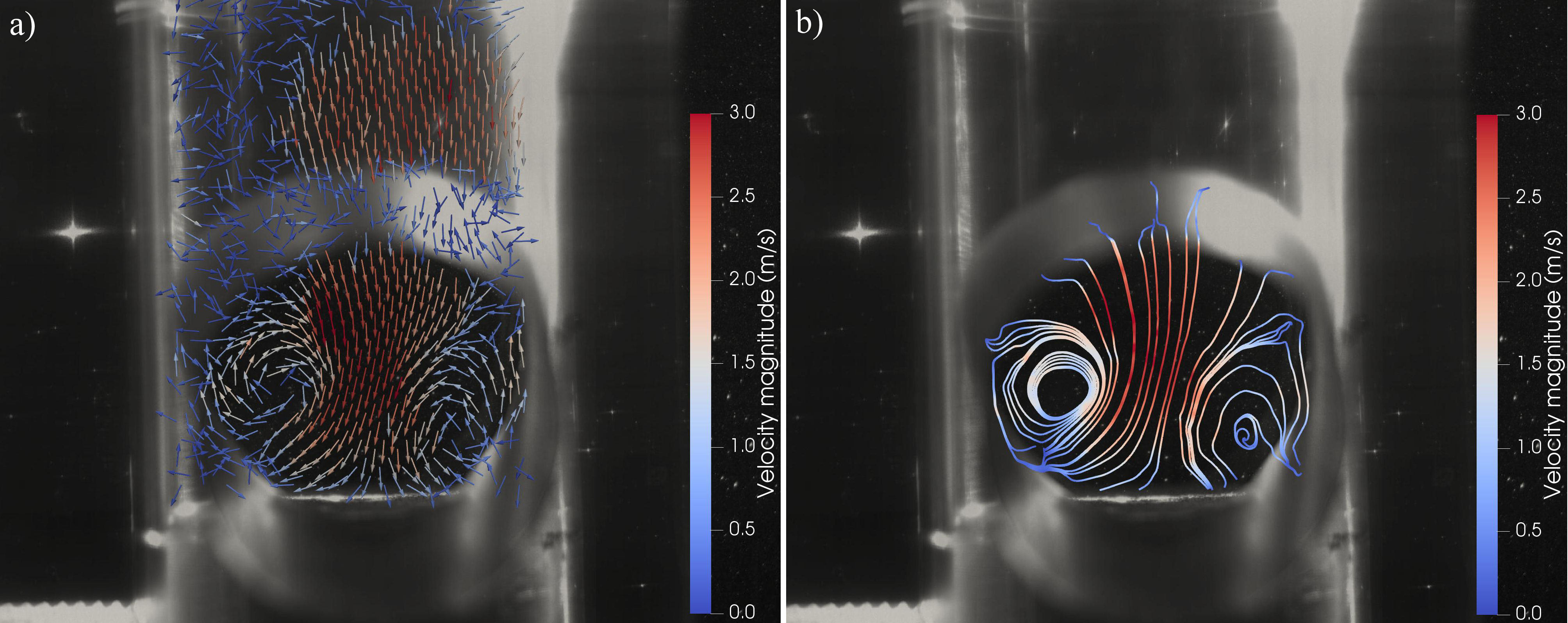
FIGURE 5 Lateral view of the right exit port of the SEN inside the visualization cell. a) Velocity vectors are superposed in the image to show the flow pattern behavior. b) Velocity magnitude streamlines superposed on the same image using PIVlab software.
Figure 5a) shows an image at 1.50 seconds of the recording experiment. At the time, the size of the vortices is almost equal, the flow swirls mostly clockwise. The observation of vectors at separate times shows that the size of both vortices changed almost at the same time, the size of the lower right vortex increased almost to one-fourth of the exit port size. The main vortex reached the total size of the exit port at different moments of the video. The main vortex position moves downward, and the lower vortex moves upward to reach the middle line of the port.
Figure 5b) shows the streamlines of the flow, obtained from the calculated vector field explained before. The streamlines help us understand that the secondary vortex located at the lower right zone of the exit port is greater than the core region. Because of the size of the vectors, it is not possible to identify their direction, but the streamlines show that the counter clockwise flow is greater than the vector observation.
The flow pattern observed in Fig. 5 did not change considerably throughout the video. This flow behavior is related to the inlet flow velocity and the size of the pool. In this case, the size of the pool is zero. In an earlier experiment reported in Real et al. work, the inlet velocity magnitude was increased and reduced by 25 percent [17]. In that experiment, the inlet velocity variations changed the flow pattern in the exit ports and affected the jet flow behavior. Significant changes were also observed when using different depths in the pool region of the SEN. The pool region reached 0.02 meters in height and the size of the vortex also increased and affected the position fluctuations at the same inlet velocity. It is worth noting that the internal flow behavior seen and measured in this work is consistent with the previously reported in literature [5,8,17].
6. Numerical analysis of the behavior in the visualization cell
To corroborate the visualization findings and to expand the discussion of the experimental results, a numerical campaign using two distinct approaches was conducted. Section 6 is divided into two, the numerical simulation results using the computational fluid dynamics, CFD technique, to solve the flow dynamics inside the SEN with the OpenFOAM software [30], and the second part of this section which reports the Smoothed Particles Hydrodynamics, SPH results. The numerical model was solved to obtain the flow pattern outside the SEN. This technique allows us to observe and analyze the jet flow behavior that exits from the SEN and discharges to a reduced volume with similar dimensions as the visualization cell. To solve the numerical model, the GPUSPH software was used. The results of this technique show that it is possible to reproduce the high turbulent flow behavior. In this qualitative analysis the SPH numerical results have multiple similarities with the physical experiments.
The CFD numerical results were compared using qualitative and quantitative information obtained from the experiments reported in this work. The SPH technique has not been reported as extensively as CFD in literature. This work proposed a qualitative comparison of the flow dynamics outside the SEN for a standard slab. The quantitative analysis of the flow dynamics of this system will be presented in further work.
6.1. Numerical analysis using CFD
In the Computational Fluid Dynamics technique (CFD) the fluid flow motion is reconstructed numerically by solving the corresponding energy and momentum transport equations. The liquid used in numerical simulations was the same as the one used in physical simulations, water, which is an incompressible fluid that displays Newtonian behavior. Since the system works continuously in relatively short time intervals, it is reasonable to assume that it operates under isothermal conditions, and so, the energy transport equation can be omitted. Therefore, the mathematical model to solve comprises only the transient Navier-Stokes equations.
Modeling the turbulent flow correctly inside the SEN is crucial for reproducing the oscillating vortices observed in the physical experiments presented in this work and previous reports. Real et al. analyzed the fluid flow patterns inside a bifurcated SEN obtained through unsteady state numerical simulations using the κ − ε and the Large Eddy Simulations (LES) turbulence models in Ref. [17]. The authors found that the κ − ε model fails to recover the oscillating behavior observed experimentally inside the SEN. Based on the previous analysis and the results presented in Shukla & Dewan [31], the transient numerical simulations presented in this work were carried out with the LES turbulence model, including the dynamic Îo-equation SGS model as scale filtering.
The OpenFOAM CFD toolbox was employed to solve the governing equations. The Pressure Implicit with Split Operator (PISO) method was employed to address the pressurevelocity coupling. The convergence criterion is fulfilled when residuals for all the modeled variables reached values equal to or less than 1×10⁻⁵ at the same time step.
The boundary conditions for the numerical model were set based on the following analysis. In physical simulations, the SEN outlet jets discharge the water into the atmosphere. Therefore, the atmospheric pressure was prescribed on the SEN exit ports. Results previously reported in literature and observations from physical simulations of this work show reverse flow sections at the exit ports. On that account, the InletOutlet boundary condition was applied to both SEN exit ports. The non-slip condition was imposed on all the SEN walls. A mapped boundary condition was set for the SEN inlet to simulate a fully developed turbulent fluid flow pattern. The average value for the inlet velocity was set as 1.150 m/s.
Numerical simulations showed that the fluid flow pattern inside the SEN changes continuously. Nevertheless, the major features of the flow pattern remain recognizable over time. Figure 6 shows the flow streamlines on a plane located in the middle of the SEN. The color of the streamline at a specific location corresponds with the fluid velocity magnitude at that point. Direct comparison of Figs. 5 and 6 shows qualitative coincidence between the hydrodynamic behavior observed and depicted with the PIV and CFD methods.
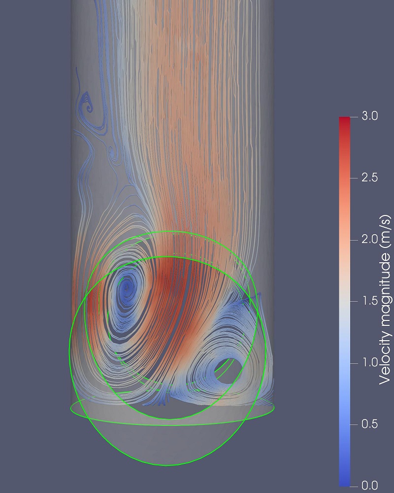
FIGURE 6 Streamlines obtained by CFD simulations colored by its velocity magnitude of the SEN internal flow at t =3.200 seconds of numerical simulation.
Figure 6 displays several vortical structures of multiple scales. One vortex, the biggest, almost occupies threequarters of the SEN bottom zone volume, the other vortex occupies the other quarter. This figure also shows that there are other smaller-scale vortices located above the biggest one. The physical simulations also showed that there are two leading vortices. The size ratio between the vortices is similar to the CFD results. The vortices’ cores are at different heights. In physical simulations, the core of the biggest vortex is slightly below the middle of the port, while in numerical simulations, the core height is almost three-quarters of the port’s height.
To quantitatively evaluate the agreement between the physical and numerical simulations, histograms of the liquid velocity magnitude on two windows of similar areas were constructed. The histograms are shown in Figs. 7a) and 7b), while the interrogation areas are shown in Figs. 7c) and 7d). Both histograms have the same scale for the liquid velocity magnitude and have the same number of intervals. The number of samples in the physical simulations and the numerical simulations is not the same. However, the trend shown by each histogram is very similar to each other.
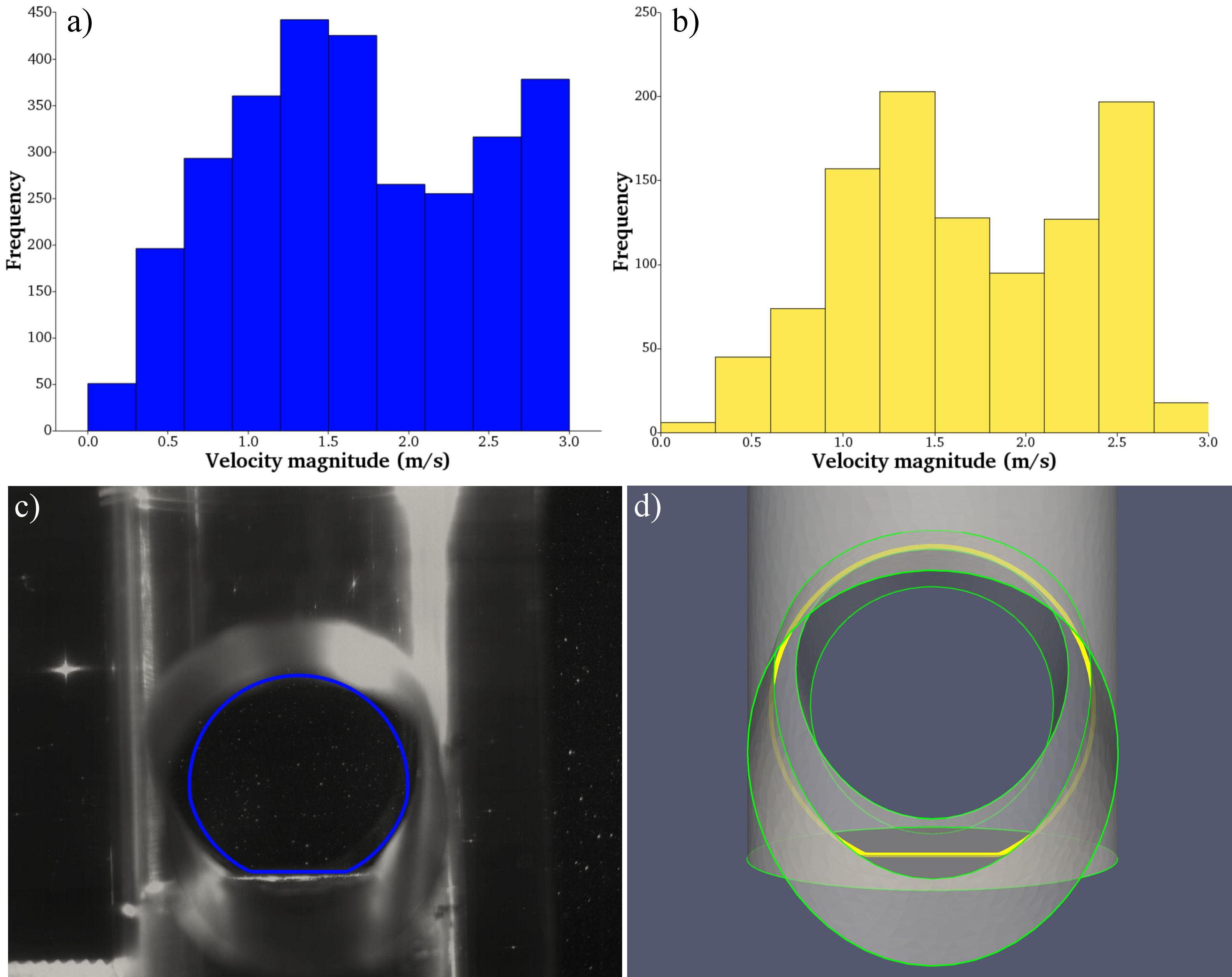
FIGURE 7 Velocity magnitude histograms and regions of interest in physical and numerical models a) Histogram obtained from experiments and b) Histogram from CFD numerical simulations. c) The circular area is defined as a region of interest to obtain the histogram in experiment and d) The circular area defined as a region of interest to obtain the histogram in CFD numerical simulations.
Qualitative similarities are found between the physical and numerical simulations on the central region of both histograms, Figs. 7a) and 7b). Due to intrinsic uncertainties of both techniques, a bias in the distribution in both histograms could also be found. In the PIV technique, the use of a laser source produces a high-intensity sheet that intensifies reflections that could affect the velocity field determination, in this case, there is high frequency in the higher velocity magnitude region. On the other hand, in numerical simulations, the boundary conditions, inlet turbulence spectrum, grid topology, and the number of elements affect the precision of the results.
6.2. Numerical analysis with smoothed particles hydrodynamics
The Smoothed Particles Hydrodynamic method is a Lagrangian, particle-based method for simulations of continuum media. Having its origins in astrophysics the method rapidly spread to applications in engineering and industry [32]. Among the advantages of the method, it can be mentioned the easy treatment of the open surfaces and complex boundaries, explicit integration of dynamic equations in a weakly compressible formulation, and the relatively simple inclusion of various physical processes. Despite its popularity in modeling both confined and free boundary flows its use in simulations of the steel casting process is still a novelty.
Recently, Gabbasov et al. have investigated the possibility of simulating the process of continuous casting using an open-source implementation of SPH code, GPUSPH [14]. It was shown that the flow structure is satisfactorily reproduced when compared with the mesh-based codes. Moreover, the numerical parameters and schemes for stable code evolution were determined.
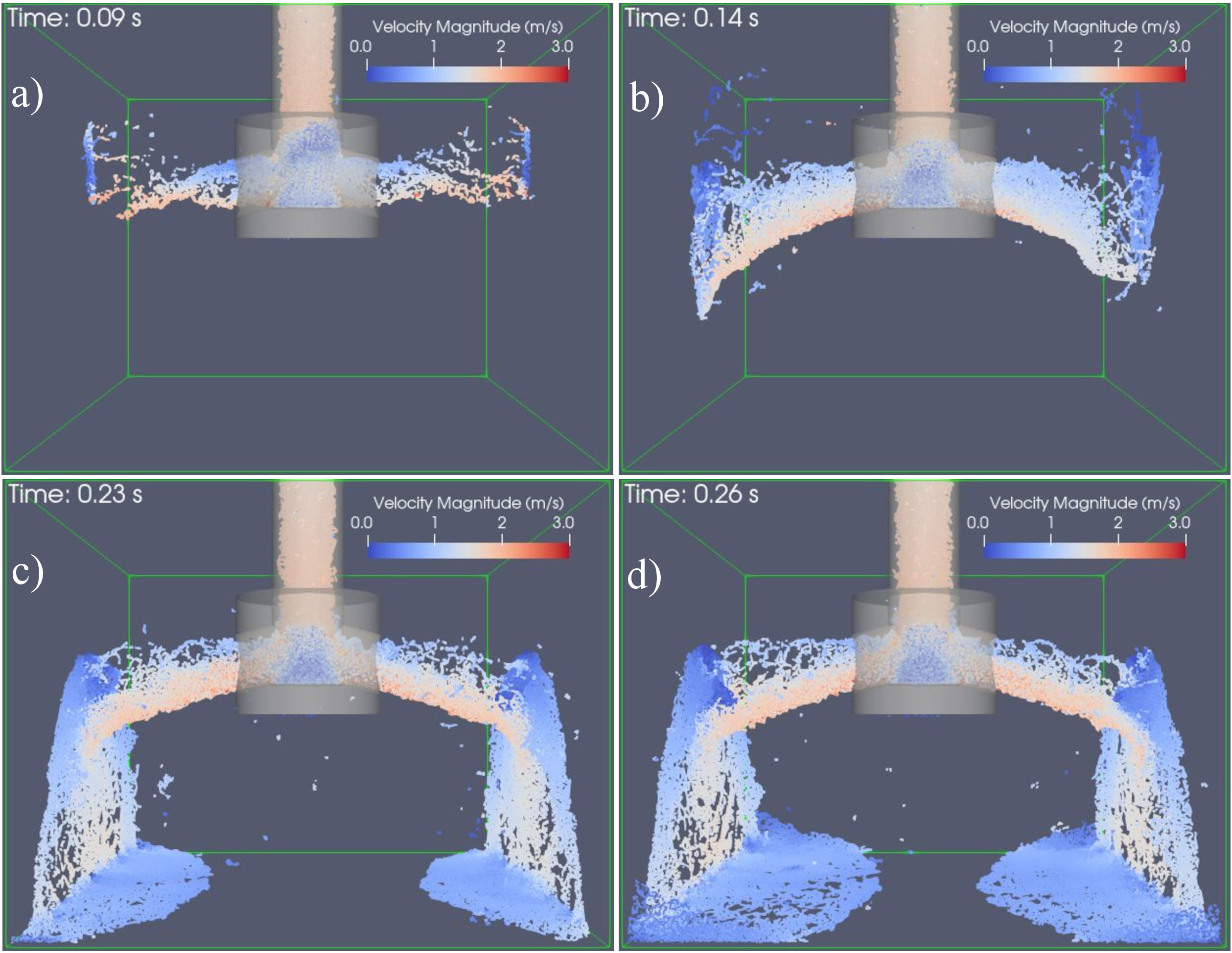
FIGURE 8 Jet flow emerging from the SEN that impinges to cell walls at different time instances using SPH technique.
In this work, we use the SPH simulations to investigate the process of jet formation and enhance the results of the previous section. The code description and relevant numerical parameters are detailed in [14]. The geometry of the SEN and visualization cell used in simulations match the experimental ones. A constant, parabolic velocity profile was imposed on the inlet with maximum velocity u max =1.15 m/s and the jets fell free into the air. The turbulence is modeled using the κ − ε turbulence model and semi-analytic boundaries are used for the walls. A detailed study of different SEN geometries and code parameters will be published in a separate paper.
In Fig. 7, four-time instants are shown depicting jets emergence and wall impingement that may be qualitatively compared to Fig. 3. These instants correspond to the transition period lasting nearly 0.25 s after which, the jet pattern is established and remains unchanged till the end of the simulation. Concerning the jet shapes, these are narrower and concentrated towards the bottom, while the jets seen in the experiment have cone shapes and have higher impingement points.
7. Conclusions
A detailed reconstruction of the fluid flow inside and outside a transparent scaled SEN model placed inside a transparent visualization cell was done in this work. Visualization and PIV techniques were used to analyze the characteristics of the internal and external flow of the SEN. CFD and SPH were the numerical techniques used to solve the internal flow pattern and the flow dynamics outside the SEN, respectively.
A qualitative comparison of the jet flow that exits through the SEN was performed between the visualization technique and the SPH numerical results. The flow downs through the inlet port and reaches the SEN lower region then interacts with the internal walls, generating a high turbulent flow zone, also the flow is divided into two streams. Finally, both streams exit the SEN through the exit ports. Once the flow exits the nozzle, it is possible to observe the asymmetry between the left and the right exit ports, because of the generated turbulence between the exit ports.
The quantitative comparison is presented between the PIV measurements and the CFD numerical simulations. Velocity magnitude histograms are obtained in a circular section inside the SEN in both models and show that the velocity field profiles are comparable. The qualitative analysis shows that it is possible to observe vortexes through the exit ports of the SEN. Their positions and numbers change periodically, there are predominantly two at the central plane of the SEN volume, or sometimes, one on the left side of the exit port. These vortices travel vertically along the SEN’s plane and determine the direction of the swirl flow at the exit ports. The non-intrusive experimental technique used in this work, PIV, contributes to the understanding of flow dynamics inside the SEN. To fully restore the fluid dynamics such results are useful for qualitative and quantitative comparisons with numerical simulations.
A novel method based on the qualitative and quantitative analysis between physical and numerical simulation results is presented in this work. This analysis will be used to examine different operational conditions and as a developmental method to design and evaluate submerged entry nozzles for a continuous casting process and other turbulent flow systems.
Fundings
This study was funded by the Instituto Politécnico Nacional, the Universidad Autónoma Metropolitana, and the Consejo Nacional de Ciencia y Tecnología.
Conflicts of interest
The author declares no conflict of interest.
Complementary material
To clarify the explanations written in Secs. 5 and 6 of this work, the authors include a full HD video named visualization.avi showing the hydrodynamic behavior inside and outside the SEN, which operates within the visualization cell.

