SciELO - Scientific Electronic Library Online

 
vol.67 número3Soliton solutions of nonlinear fractional differential equations with their applications in mathematical physicsFactorization method for some inhomogeneous Liénard equations índice de autoresíndice de assuntospesquisa de artigos
Home Pagelista alfabética de periódicos  

Serviços Personalizados

Journal

Artigo

Indicadores

Links relacionados

  • Não possue artigos similaresSimilares em SciELO

Compartilhar


Revista mexicana de física

versão impressa ISSN 0035-001X

Rev. mex. fis. vol.67 no.3 México Mai./Jun. 2021  Epub 21-Fev-2022

https://doi.org/10.31349/revmexfis.67.429 

Research

Gravitation, Mathematical Physics and Field Theory

A two-index generalization of conformable operators with potential applications in engineering and physics

1Departamento de Física y Matemáticas, Universidad Iberoamericana, Ciudad de México, México. e-mail: rceduardo1l@gmail.com;

2Departamento de Física y Matemáticas, Universidad Iberoamericana, Ciudad de México, México. e-mail: guillermo.fernandez@ibero.mx;

3Instituto de Ciencias Físicas, Universidad Nacional Autónoma de México, Av. Universidad s/n Col. Chamilpa, 62210 Cuernavaca, Morelos, México. e-mail: jchavez@icf.unam.mx;

4Facultad de Física. Universidad de La Habana, La Habana, Cuba. Departamento de Física y Matemáticas, Universidad Iberoamericana, Ciudad de México, México. e-mail: leovildo.diago@ibero.mx;

5Universidad Autónoma de la Ciudad de México, Fray Servando Teresa de Mier 92, Col. Centro, Alcaldía Cuauhtémoc, CDMX, México 06080 e-mail: rodrigo.munoz@uacm.edu.mx;


Abstract

We developed a somewhat novel fractional-order calculus workbench as a certain generalization of Khalil’s conformable derivative. Although every integer-order derivate can naturally be consistent with fully physical-sense problem’s quotation, this is not the standard scenario of the non-integer-order derivatives, even aiming physics systems’ modeling, solely. We revisited a particular case of the generalized conformable fractional derivative and derived a differential operator, whose properties overcome those of the integer-order derivatives, though preserving its clue advantages. Worthwhile noting that the two-fractional indexes differential operator we are dealing with departs from the single-fractional index framework, which typifies the generalized conformable fractional derivative. This distinction leads to proper mathematical tools, useful in generalizing widely accepted results, with potential applications to fundamental Physics within fractional order calculus. The latter seems to be especially appropriate for exercising the Sturm-Liouville eigenvalue problem, as well as the Euler-Lagrange equation, and to clarify several operator algebra matters.

Keywords: Conformable operators; algebraic methods; quantum operators; sturm Liouville operator

1.Introduction

Derivatives of non-integer order have been discussed for a long time. In 1695 L’Hôpital asked Leibniz what meaning could be ascribed to Dnf if n were a fraction. Since that time, fractional calculus has drawn the attention of many mathematicians. Most of them have used an integral form to define the fractional derivative; the two most popular ones are the Riemann-Liouville definition and the Caputo definition. However, these definitions did not inherit most of the properties of the classic integer-order derivative, such as the product rule or the chain rule. In 2014 Khalil et al. 1 introduced the definition of the conformable fractional derivative, analogous to the limit definition of the standard integer-order derivative. This definition was later generalized by Katugampola 2, whose work was later addressed by Anderson et al. 3, who used Katugampola’s results to explore its properties and its potential application in quantum mechanics, see also 4-8. In 2017, Al-Refai and Abdeljawad 9 suggested a generalization of the well-known Sturm-Liouville eigenvalue problem using the conformable derivative. In 2018 Zhao et al. 10 introduced a set of Maxwell’s equations using the Generalized Conformable Fractional Derivative (GCFD), which obeys the classical properties of the integer-order derivative. Several works have recently appeared on conformal derivatives, e.g., 14-19. Clearly showing that it is a field of great growth, despite its recent creation. Some applications of these conformal derivatives to optical solitons solutions are in 20,21.

We generalize the conformable derivative introduced by Khalil et al. 1 by exploring the properties of a fractional derivative operator derived from the GCFD derivative. Unlike the rest of the fractional derivatives, the order of our operator is determined by two fractional indexes and two positive functions, which can be arranged to recover the integer order derivative. The two fractional indexes and the two functions give the derivative greater freedom and more complex dynamics than single-index and single-function derivatives; furthermore, being a conformable derivative, it is a local derivative just like in the integer-order case. In this way, our proposed GCFD is similar to the Gateaux derivative 10 but definitively is not equal. We present a differential operator in which the order of the derivative now depends on the two fractional indexes α and β, preserving almost all the properties of integer-order derivatives, as it is often the case with conformable local derivatives. We construct operators with potential application in quantum mechanics, generalizing some results obtained by Anderson and Ulness 3. We generalize some well-known results, such as the Euler-Lagrange method 11 and the Sturm-Liouville eigenvalue problem 12 by replacing the integer-order derivative operators with our operator, following a similar procedure as Abdeljawad et al. 9 and we show some examples.

In the first section, we present the definition of the operator, its main properties, such as the product rule and the chain rule, as well as some examples. In the next section, we further explore its properties, we introduce an inverse operator, and then we explore its commutator and anti-commutator properties, as well as some results with applications in quantum mechanics. In the last section, we generalize some results obtained in the second section, namely the Sturm-Liouville operator. We consider the Sturm-Liouville eigenvalue problem using the differential operator introduced in the first section. We also generalize some results, such as the Lagrange Identity and the Euler-Lagrange equation.

2.Preliminaries

Let ψ(u,α,β) be a fractional conformable function and α,β (0,1]. The “αβ derivative” of f: R+R at x is defined as:

Dψα,β(f)(x)=limϵ0f(x+ϵψ(x,α,β))-f(x)ϵ. (1)

The restrictions of ψ(u,α,β) are:

ψ(x,1,1)=1x  R+ψ(x,α,β)0x  R+ψ(.,α1,β)ψ(.,α2,β)α1α2ψ(.,α,β1)ψ(.,α,β2)β1β2

where αi and βi (0,1], for i =1, 2, 3…. Let f: [0, ] ,R and x > 0 also let h(x) and k(x) be continuous functions, where h(x)>0 and k(x)>0. Then the “α,βhkl conformable fractional derivative” of f of order α, β is defined by:

Dh,k,lα,β(f)(x)=limϵ0f(x+hβ(x)elϵk1-α(x))-f(x)ϵ, (2)

where

elϵk1-α(x)=j=1lϵjk(1-α)j(x)j!, (3)

for x > 0, α,β (0,1]. If the limit exists, we say that f (x) is γ-differentiable.

Recently M.N. Alam and Xin Li 13 solved the complex fractional Schrödinger equation using the conformable derivative introduced by Khalil et al. 1; our fractional operator generalizes the operator introduced by Khalil.

If we set h(x)=1, β = 1, k(x)=x and l =1 then we recover the conformable fractional derivative definition from Khalil et al.:

D1,t,1α,1(f)(x)=limϵ0f(x+ϵx1-α)-f(x)ϵ. (4)

If we set h(x) = x, β = 1, k(x)=xαα-1 and l then we recover the fractional derivative of order α definition from Katugampola:

Dx,xαα-1,α,1fx=limϵ0fxeϵx-αx-fxϵ (5)

3.Properties of the differential operator

Let α (0,1] and f,g be γ -differentiable at a point x > 0. Using (2) and (2), it can be easily proved that:

  1. Dh,k,lα,β(af+bg)=aDh,k,lα,β(f)+bDh,k,lα,β(g), α, b R.

  2. Dh,k,lα,β(xn)=nxn-1hβ(x)k1-α(x), n R.

  3. Dh,k,lα,β(c)=0, for all constant functions.

  4. Dh,k,lα,β(fg)=g(x)Dh,k,lα,β(f)+f(x)Dh,k,lα,β(g).

  5. Dh,k,lα,β(fg)=g(x)Dh,k,lα,β(f)-f(x)Dh,k,lα,β(g)g2(x).

  6. Dh,k,lα,β(fg)=dfdx(g(x))Dh,k,lα,β(g)(x).

  7. Dh,k,lα,β(f)=hβ(x)k1-α(x)dfdx.

  8. Dh,k,lα,βf(y1(x),...,yN(x))=fy1Dh,k,lα,β(y1)+...+fyNDh,k,lα,β(yN).

4.The αβhkl conformable fractional derivate and its relationship with second-order linear defferential equations

We now further explore the properties of our differential operator (2) and develop some new operators from this one, such as the inverse operator, the commutator and the anti-commutator as well as a self-adjoint variant of the anti-commutator. We will later use some of this results when solving the Sturm-Liouville eigenvalue problem, such as the integration by parts formula.

4.1.The Dh,k,lα,β operator

We begin by exploring the properties of the Dh,k,lα,β operator.

Dh,k,lα,β[y(x)]=hβ(x)k1-α(x)dy(x)dx, (6)

where d/dx is the integer-order derivative operator. So the Dh,k,lα,β operator is

Dh,k,lα,β=hβ(x)k1-α(x)ddx. (7)

Next, we considered the iterated operator Dh,k,lα,βDh,k,lρ,σ

Dh,k,lα,β[Dh,k,lρ,σy]=hβxk1-αxddx[hσxk1-ρxy']=hβ(x)k1-α(x)(σhσ-1(x)h'(x)×k1-ρ(x)y'+(1-ρ)hσ(x)k-ρ(x)×k'(x)y'+hσ(x)k1-ρ(x)y).

If we let γ1=α+β and γ2=β+σ, then:

=hγ2(x)k2-γ1(x)y+(σhγ2-1(x)h'(x)×k2-γ1(x)+(1-ρ)hγ2(x)k1-γ1(x)×k'(x))y'. (8)

4.2.The operator Ih,k,lα,β

We define the inverse operator of Dh,k,lα,β as

(Dh,k,lα,β)-1Ih,k,lα,β=x(.)kα-1(t)h-β(t)dt=x(.)dγ(t), (9)

where (.) is a place holder for the function to be operated upon.

Applying the anti-derivative operator Ih,k,lα,β to Dh,k,lα,β yields

Ih,k,lα,β[Dh,k,lα,β[y]]=xy(t)dγ(t)=y(x), (10)

where one takes y to vanish at the lower limit. Now applying the Dh,k,lα,β operator to Ih,k,lα,β yields

Dh,k,lα,β[Ih,k,lα,β[y]]=Dh,k,lα,β[xy(t)dγ(t)]=hβ(x)k1-α(x)ddx×[xy(t)dγ(t)]=y(x). (11)

However, in the mixed case Dh,k,lρ,σIh,k,lα,β yields:

Dh,k,lρ,σ[Ih,k,lα,βy]=Dh,k,lρ,σ[xytytdγt]=hσxk1-ρxddx[xytdγt],

let δ1=α-ρ and δ2=σ-β

=hδ2(x)kδ1(x)y(x). (12)

Similarly for Ih,k,lα,βDh,k,lρ,σ we have

Ih,k,lα,β[Dh,k,lρ,σ[y]]=xkα-1(t)h-β(t)hσ(t)k1-ρ(t)y'dt=xkδ1(t)hδ2(t)y'(t)dt=hδ2(x)kδ1(x)y(x)-δ1xkδ1-1(t)k'(t)hδ2(t)y(t)dt-δ2xhδ2-1(t)h'(t)kδ1(t)y(t)dt=hδ2(x)kδ1(x)y(x)\na-δ1Ih,k,lδ1,δ2[h2δ2(x)k'(x)y(x)]-δ2Ih,k,lδ1,δ2[h2δ2-1(x)h'(x)k(x)y(x)]. (13)

Using the definition for the anti-derivative operator, we can also derive a formula for integration by parts.

Theorem 4.1 (Integration by parts)

Let f,g:[a,b]Rbe two functions such thatfgis differentiable, then:

abfxDh,k,lα,βgxdγx=fxgx|ab-abg(x)Dh,k,lα,βg(x)dγ(x) (14)

proof

abfxDh,k,lα,βgxdγx=abfxhβxk1-αxg´x×dγx=fxgx|ab-abgxf´xdx=fxgx|ab-abgxhβxk1-αxf´xh-βxka-1xdx=fxgx|ab-abg(x)Dh,k,lα,βf(x)dγ(x)

4.3.Parity in the Dh,k,lα,β operator

We can neglect the requirement that t > 0 and consider the parity of Dh,k,lα,β by applying the operator Pˆ on (7):

P^Dh,k,lα,β=P^[hβk1-α(x)ddx]=hβ(-x)k1-α(-x)(-ddx). (15)

We may consider two cases for powers of h(x) and k(x) of the form:

ν1=12n+1, (16)

and

ν2=2n2n+1, (17)

where nZ0

So, the action of Pˆ becomes:

PˆDh,k,l1-νi,νj=hνj(-x)kνi(-x)-ddx, (18)

where i,j=1,2. Taking into account the parity of h(x) and k(x), we explore the different cases for Pˆ:

4.3.1. v 1

1.

P^Dh,k,l1-ν1,ν1=h12n+1(-x)k12n+1(-x)(-ddx), (19)

(1) h(x) even and k(x) even or h(x) odd and k(x) odd

PˆDh,k,l1-ν1,ν1=eiπDh,k,l1-ν1,ν1, (20)

(2) h(x) even and k(x) odd or h(x) odd and k(x) even

PˆDh,k,l1-ν1,ν1=Dh,k,l1-ν1,ν1. (21)

4.3.2. v 2

1.

P^Dh,k,l1-ν2,ν2=h12n+1(-x)k12n+1(-x)(-ddx). (22)

(1) h(x) even and k(x) even or h(x) odd and k(x) odd or h(x) even and k(x) odd or h(x) odd and k(x) even

PˆDh,k,l1-ν2,ν2=eiπDh,k,l1-ν2,ν2. (23)

4.3.3. v1 and v2

P^Dh,k,l1-ν2,ν1=h12n+1(-x)k22n+1(-x)(-ddx), (24)

(1) h(x) even and k(x) even or h(x) even and k(x) odd

PˆDh,k,l1-ν2,ν1=eiπDh,k,l1-ν2,ν1, (25)

(2) h(x) odd and k(x) even or h(x) odd and k(x) odd

PˆDh,k,l1-ν2,ν1=Dh,k,l1-ν2,ν1. (26)

2.

P^Dh,k,l1-ν1,ν2=h22n+1(-x)k12n+1(-x)(-ddx), (27)

(1) h(x) even and k(x) even or h(x) odd and k(x) even

PˆDh,k,l1-ν1,ν2=eiπDh,k,l1-ν1,ν2, (28)

(2) h(x) even and k(x) odd or h(x) odd and k(x) odd

PˆDh,k,l1-ν1,ν2=Dh,k,l1-ν1,ν2. (29)

4.4.First order differential equation

We consider a differential equation for the Dh,k,lα,β operator:

Dh,k,lα,β[y(x)]+λy(x)=0. (30)

Using (6) and solving for y(x):

hβ(x)k1-α(x)y'(x)+λy(x)=0y'(x)+λh-β(x)kα-1(x)y(x)=0ddx[eλxh-βtkα-1t\dityx]=0y(x)=ce-λxh-β(t)kα-1(t)\dit.

4.5.The commutator with the Dh,k,lα,β derivative

The operators Dh,k,lα,β and Dh,k,lα,β do not commute, and unlike integer-order derivatives Dh,k,lα,βDh,k,lα,βDk,lα+ρ,β+σ; however, it is interesting to explore the commutator properties of these operators.

[Dh,k,lα,β,Dh,k,lα,β]y=Dh,k,lα,β[Dh,k,lα,βy]-Dh,k,lρ,σ[Dh,k,lα,βy].

From (8):

=((σ-β)hβ+σ-1(x)h'(x)k2-α-ρ(x)+(α-ρ)hβ+σ(x)k1-α-ρ(x)k'(x))y'=(δ2hγ2-1(x)h'(x)k2-γ1(x)+δ1hγ2(x)×k1-γ1(x)k'(x))y' (31)

Since γ1=α+ρ,γ2=β+σ,δ1=α-ρ,δ2=σ-β.

Dh,k,lα,β,Dh,k,lα,β=0 (32)

and

Dh,k,lα,β,Dh,k,lρ,σ=-Dh,k,lα,β,Dh,k,lρ,σ (33)

Using the result from (31):

[Dh,k,la,b,[Dh,k,lc,d,Dh,k,lm,n]]y=Dh,k,la,b[Dh,k,lc,d,Dh,k,lm,n]y-[Dh,k,lc,d,Dh,k,lm,n]Dh,k,la,b[y]=k-a-c-m+1(x)(-hb+d+n-2(x))×(h2(x)(a2+a(m-2)-m(c+m)+c+m)[k'(x)]2y'(x)+h(x)k(x)(y'(x)((m-a)h(x)\ntk(x)-h'(x)k'(x)(b(2a+m-3)+n(a-c-2m+2)+d×(-m)+d))+h(x)(-2a+c+m)k'(x)y(x))+k2(x)(y'(x)((b2+b(n-1)-n(d+n)+n)×h']2x+b-nhxhx +h(x)(2b-d-n)h'(x)y(x))). (34)

Then, we can verify that the Jacobi identity holds:

Dh,k,la,b,Dh,k,lc,d,Dh,k,lm,n+Dh,k,lc,d,Dh,k,lm,n,Dh,k,la,b+Dh,k,lm,n,Dh,k,la,b,Dh,k,lc,d=0 (35)

If we consider the commutator [Dk,lα,t] acting on a function y(x):

[Dh,k,lα,β,x]y=Dh,k,lα,β[xy]-xDh,k,lα,β[y]=xDh,k,lα,β[y]+yDh,k,lα,β[x]-xDh,k,lα,β[y]=hβ(x)k1-α(x)y. (36)

Thus

Dh,k,lα,β,x=hβ(x)k1-α(x) (37)

Then, we can express the generalized conformable fractional derivative acting on y as

Dh,k,lα,βy=Dh,k,lα,β,xy´ (38)

So, for any differentiable function of x:

Dh,k,lα,β,f(x)=hβxk1-αxf´(x) (39)

Using Eq.(12) and Eq.(13), we can consider the commutator [Ik,lα,Dk,lβ]

[Ih,k,lα,β,Dh,k,lρ,σ]y=-δ1Ih,k,lδ1,δ2[h2δ(x)k'(x)y]-δ2Ih,k,lδ1,δ2[h2δ2-1(x)h'(x)k(x)y]. (40)

4.6.The anti-commutator for the operator Dh,k,lα,β

We now consider the anti-commutator by defining the operator

C^γ1,γ212{Dh,k,lα,β,Dh,k,lρ,σ}=12(Dh,k,lα,βDh,k,lρ,σ+Dh,k,lρ,σ,Dh,k,lα,β). (1)

Using Eq.(8) and operating Cˆγ on a function y(x):

C^γ1,γ2y=12(hγ2(x)k2-γ1(x)y+(σhγ2-1(x)h'(x)k2-γ1(x)+(1-ρ)hγ2(x)k1-γ1(x)k'(x))y')+12(hγ2(x)k2-γ1(x)y+(βhγ2-1(x)h'(x)k2-γ1(x)+(1-α)hγ2(x)k1-γ1(x)k'(x))y')=hγ2(x)k2-γ1(x)y+12(γ2hγ2-1(x)h'(x)k2-γ1(x)+(2-γ1)hγ2(x)k1-γ1(x)k'(x))y'. (42)

We may consider the case when α = p and β = σ, then,

C^2α,2βy=12{Dh,k,lα,β,Dh,k,lα,β}=(Dh,k,lα,β)2. (43)

If α=β=1/2:

C^1,1y=h(x)k(x)y+12(h'(x)k(x)-h(x)k'(x))y'. (44)

4.6.1.Some properties for Cˆγ1,γ2y

Lets first consider the homogeneous equation for α = p and β = σ,

Cˆ2α,2βy=0. (45)

Then Eq.(42) becomes:

h2β(x)k2-2α(x)y+(βh2β-1(x)h'(x)k2-2α(x)+(1-α)h2β(x)k1-2α(x)k'(x))y'=0, (46)

which has solution:

y(x)=C2+xC1h-β(t)kα-1(t)dt. (47)

Lets now consider the constant equation

C2α,2βˆy=Λ. (48)

Equation Eq.(42) becomes

x2k-2α(x)y+(tk-2α(x)-αx2k-(2α+1)(x))y'=Λ, (49)

which has the solution:

y(x)=c2+x(c1exαs2-k(s)sk(s)s2ds+exαs2-k(s)sk(s)s2ds×xezαs2-k(s)sk(s)s2dsΛk2α(z)z2dz)dt, (50)

where c1 and c2 are constants to be determined by boundary conditions.

4.6.2.Self-adjoint operator of Cˆ2α,2β

The operator Cˆ2α,2β is not self-adjoint, but it can be made so by multiplying by an integrating factor W(x),

W(x)=1h2β(x)k2-2α(x)×exβh2β-1(x)h'(x)k2-2α(x)+(1-α)h2β(x)k1-2α(x)k'(x)h2β(x)k2-2α(x)dx=1h2β(x)k2-2α(x)exβh'(x)h(x)+(1-α)k'(x)k(x)dx=h-β(x)kα-1(x). (51)

We define:

A^2α,2βW(x)C^2α,2β=(h-β(x)kα-1(x))h2β(x)k2-2α(x)×d2dx2+[βh2β-1(x)h'(x)k2-2α(x)+(1-α)h2β(x)k1-2α(x)k'(x)]ddx=hβ(x)k1-α(x)d2dx2+(βhβ-1(x)h'(x)×k1-α(x)+(1-α)hβ(x)k-α(x)×k'(x))ddx=ddxhβ(x)k1-α(x)ddx. (52)

4.6.3.Differential equations for Aˆ2α,2β

Now that we have defined Aˆ2α,2β, we solve two differential equations using this operator.

1.Homogeneous equation

Aˆ2α,2βy=0, (53)

which solution is:

y(x)=c1xh-β(s)kα-1(s)ds+c2, (54)

where c1 and c2 are constants to be determined by boundary conditions.

2.Equation including a constant inhomogeneous term

A^2α,2βy=κ, (55)

y(x)=1x(c1+κs)h-β(s)kα-1(s)ds+c2, (56)

where c1 and c2 are constants to be determined by boundary conditions, and κ is a constant term.

Example:

Setting h(x)=xm and k(x)=xn, yields the solution:

y(x)=c1x1+n(α-1)-mβ1+n(α-1)-mβ+κx2+n(α-1)-mβ2+n(α-1)-mβ+c2, (57)

where n,m Z>0.

We can re-express this solution in the from:

yG,q1,q2,q3(x)=q1(α,β,m,n)xG(α,β,m,n)+q2(α,β,m,n)x1+G(α,β,m,n)+q3, (58)

where:

G(α,β,m,n)=1+n(α-1)-mβ (59)

q1(α,β,m,n)=c1G1(α,β,m,n) (60)

q2(α,β,m,n)=κ1+G(α,β,m,n) (61)

q3(α,β,m,n)=c2. (62)

By the law of trichotomy, Eq. (58) leaves us only with three non-singular solutions of the form:

  1. G(α,β,m,n)<1+G(α,β,m,n)<0,

  2. G1(α,β,m,n)<0<1+G(α,β,m,n),

  3. 0<G(α,β,m,n)<1+G(α,β,m,n) .

The next table shows some cases of these solutions of Eq.(58):

(1)Figure 1a), obtained by setting α=0.5, β = 0.8, m = 3, n = 2, c1 = 1, c2 = 1, κ=0, has an asymptotic behaviour determined by the value of c2, which is indicated by the dotted line.

Figure 1 Plots of different values of α, β, m, n, c1, c2, and κ for Eq. (58). 22

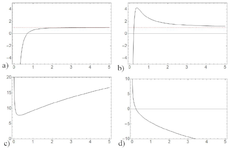
(2)Figure 1b), obtained by setting α = 0.5, β = 0.8, m = 1, n = 2, c1 = 1, c2 = 1, κ=-2.7, has an asymptotic behaviour determined by the value of c2, which is indicated by the dotted line and the maximum value of the function is determined by the value c1.

(3)Figure 1c), obtained by setting α = 0.7, β = 0.3, m = 3, n = 2, c1 = -1, c2 = 0.2, κ=3.5. In this case, the function diverges to + both at x = 0 and at x .

(4)Figure 1d), obtained by setting α = 0.7, β = 0.3, m = 3, n = 2, c1 = 0.5, c2 = 0.5, κ=-3. The function now diverges to + at x = 0 and to - at x-.

For G>0 is an interesting family of elemental functions since:

  • The value x = 0 is a local minimum or maximum in the domain ℝ + ⋃{0}.

  • By extending the domain to negative numbers, the function takes complex values, it becomes multi-valued and the concept of maximum, and minimum no longer makes sense.

  • At least the first two derivatives are null in the minimum x = 0.

  • When G = N is a natural positive exponent, the yC in R+{0}. When G is not a natural number, there is a first non-null derivative a x = 0, which is infinite.

By setting c1=-2.5, c2 = 0, κ=17.5, n = m = 1, α = 0.3, β = 0.5 in Eq.(57), we get:

y(x)=q1xG1+q2x1+G1+q3, (1)

y(x)=-x2.5+5x3.5, (64)

which is an interesting example of an elementary function (see Fig. 2).

Figure 2 Plot of Eq. (64). 22

5.Results of the Dh,k,lα,β derivative for the Sturm-Liouville eigenvalue problem

We consider the fractional extension of the Sturm-Liouville eigenvalue problem.

Dh,k,lα,βpxDh,k,lα,βyx+qxyx=-λwxyx, 0<α1, 0<β1,a<x<b (65)

where p, Dh,k,lα,β p, q and the weight functions w are continuous on (a,b),p(x)>0, and w(x)>0, on [a,b], and the fractional derivative Dh,k,lα,β is the generalized conformable fractional derivative. We consider Eq.(65) with boundary conditions

c1y(a)+c2y'(a)=0,c12+c22>0, (1)

r1y(b)+r2y'(b)=0,r12+r22>0. (67)

If Dh,k,lα,β,Dh,k,lα,βy is continuous on [a,b], then we say that y is 2γ-continuously differentiable on [a,b]. Let

Lh,k,lα,βy=Dh,k,lα,βp(x)Dh,k,lα,βy(x)+q(x)y(x) (68)

Then we may write the fractional Sturm-Liouville eigenvalue problem as

Lh,k,lα,βy=-λw(x)y(x) (69)

Theorem 5.1 (New Lagrange identity) .

Letting 𝑦 1 , 𝑦 2 be 2γ-continuously differentiable on [a,b], then the following holds:

ab(y2Lh,k,lα,β(y1)-y1Lh,k,lα,β(y2))dγ(x)=[p(x)(y2Dh,k,lα,βy1-y1Dh,k,lα,βy2)]|abf(x)|ab. (70)

proof

Let F4x,α,β=y2Lh,k,lα,βy1-y1y2Lh,k,lα,β(y2), then:

abF4(x,α,β)dγ(x)=aby2Dh,k,lα,βpxDh,k,lα,βy1dγx-aby1Dh,k,lα,βpxDh,k,lα,βy2dγx=pxy2Dh,k,lα,βy1|ab-abpxDh,k,lα,βy1Dh,k,lα,βy2dγx-pxy1Dh,k,lα,βy2|ab+abpxDh,k,lα,βy1Dh,k,lα,βy2dγx=[pxy2Dh,k,lα,βy1-y1y2]|ab.

Lemma 5.2

Let y 1 and y 2 in C1[a,b], which satisfy the boundary conditions (66) and (67). Then it holds that:

[p(x)(y2Dh,k,lα,βy1-y1Dh,k,lα,βy2)]|ab=0. (71)

Proof.

Let F5x,α,β=p(x)y2Dh,k,lα,βy1-y1Dh,k,lα,βy2, then:

F5(x,α,β)|ab=p(b)y2(b)Dh,k,lα,βy1(b)-y1(b)Dh,k,lα,βy2(b)-p(a)y2(a)Dh,k,lα,βy1(a)-y1(a)Dh,k,lα,βy2(a). (72)

Since c12+c22>0 and r12+r22>0, we first assume that c10 and r10, then:

y(a)=-c2c1y'(a), (73)

y(b)=-r2r1y'(b). (74)

Thus

y2(b)Dh,k,lα,βy1(b)-y1(b)Dh,k,lα,βy2(b)=-r2r1×y2'(b)hβ(b)k1-α(b)y1'(b)-y1'(b)hβ(b)k1-α(b)y2'(b)=0, (75)

y2(a)Dh,k,lα,βy1(a)-y1(a)Dh,k,lα,βy2(a)=-c2c1×y2'(a)hβ(a)k1-α(a)y1'(a)-y1'(a)hβ(a)k1-α(a)y2'(a)=0. (76)

Definition 1. We say that f and g are γ-orthogonal with respect to the weight function μ(x)0, if

abfxμxgxdγx=0. (77)

Theorem 5.3

The eigenfunctions of the fractional eigenvalue problem (65,66,67) corresponding to distinct eigenvalues are γ-orthogonal with respect to a weight function w(x).

Proof.

Let λ1 and λ2 be two distinct eigenvalues, and y 1 and y 2 are the corresponding eigenfunctions, then

Lh,k,lα,β(y1)=-λ1w(x)y1, (78)

Lh,k,lα,β(y2)=-λ2w(x)y2, (79)

y2Lh,k,lα,β(y1)-y1Lh,k,lα,β=-(λ1-λ2)w(x)y1y2, (80)

-(λ1-λ2)abw(x)y1y2dγ(x)=aby2Lh,k,lα,βdγ(x)-aby1Lh,k,lα,βdγ(x). (81)

From the New Lagrange identity Eq.(70) and Lemma 5.2, Eq.(71):

(λ1-λ2)abw(x)y1y2dγ(x)=0. (82)

Since λ1 λ2

abw(x)y1y2dγ(x)=0. (83)

Theorem 5.4

The eigenvalues of the fractional eigenvalue problem (65,66,67) are real.

Proof. Let y be a solution of the fractional Sturm-Liouville eigenvalue problem. Taking the complex conjugate of Eq.(68) and Eq.(69) and using the fact that p(x), q(x), and w(x) are real-valued functions, we have:

Lh,k,lα,βy-=Dh,k,lα,β(p(x)Dh,k,lα,βy-)+q(x)y¯=-λw(x)y¯, (84)

c1y¯(a)+c2y'¯(a)=0, (85)

r1y¯(a)+r2y'¯(b)=0, (86)

y¯Lh,k,lα,β(y)-yLh,k,lα,βy-=-(λ-λ¯)w(x)yy¯-(λ-λ¯)w(x)y(x)2. (87)

Then, from Lemma 5.2, Eq.(71) and Theorem 5.3,

(λ-λ¯)abw(x)y(x)2\diγ(x)=0. (1)

Thus

λ=λ¯. (89)

Definition 2.

Let f and g be γ-differentiable. The new Wronskian function is defined by

Wh,k,lα,βf,g=fDh,k,lα,βg-gDh,k,lα,βf (90)

Theorem 5.5

Let y 1 and y 2 be 2γ- continuously differentiable on [a,b]; they are linearly independent solutions of ([eq:5.1]), then:

Wh,k,lα,βy1,y2=Dh,k,lα,β(y1y2)(a)p(a)p(x) (91)

Proof.

Dh,k,lα,βWh,k,lα,β(y1y2)=Dh,k,lα,β[y1Dh,k,lα,βy2-y2Dh,k,lα,βy1]=y1Dh,k,lα,βDh,k,lα,βy2+Dh,k,lα,βy1Dh,k,lα,βy2-y2Dh,k,lα,βDh,k,lα,βy1-Dh,k,lα,βy1Dh,k,lα,βy2=y1Dh,k,lα,βy2-y2Dh,k,lα,βDh,k,lα,βy1. (92)

Analogously, applying the product rule to Eq. (65)

Dh,k,lα,βDh,k,lα,βy=-1pDh,k,lα,βpDh,k,lα,βy+(q+λw)y. (93)

Substituting into Eq.(92):

Dh,k,lα,βWh,k,lα,β(y1,y2)=-y1pDh,k,lα,βpDh,k,lα,βy2+q+λwy2+y2p(Dh,k,lα,βpDh,k,lα,βy1+(q+λw)y1)=-Dh,k,lα,βpp(y1Dh,k,lα,βy2-y2Dh,k,lα,βy1)=-Dh,k,lα,βppDh,k,lα,β(y1,y2). (94)

Solving the differential equation,

Wh,k,lα,βy1,y2=cp (95)

Then:

Wh,k,lα,βy1,y2a=cpa. (96)

Thus:

Wh,k,lα,βy1y2=Wh,k,lα,β(y1,y2)(a)p(a)p(x)

Theorem 5.5

The eigenvalues of the fractional eigenvalue problem (65, 66, 67) are simple.

Proof. Let y1 and y2 be two eigenfunctions for the same eigenvalue λ:

y2Lh,k,lα,β(y1)-y1Lh,k,lα,β=-(λ-λ)w(x)y1y2, (97)

y2L(y1,α)-y1L(y2,α)=0. (98)

From Eq.(70)

y2Dh,k,lα,β(p(x)Dh,k,lα,βy1)-y1Dh,k,lα,β(p(x)Dh,k,lα,βy2)=0. (99)

Using the fractional product rule and factoring terms:

p(x)(y2Dh,k,lα,βDh,k,lα,βy1-y1Dh,k,lα,βDh,k,lα,βy2)+Dh,k,lα,βp(x)(y2Dh,k,lα,βy1-y1Dh,k,lα,βy2)=0  Dh,k,lα,β(p(x)[y2Dh,k,lα,βy1-y1Dh,k,lα,βy2])=p(x)[y2Dh,k,lα,βy1-y1Dh,k,lα,βy2]=c. (100)

Since y1 and y2 satisfy the same boundary conditions, c=0

y2Dh,k,lα,βy1-y1Dh,k,lα,βy2=0 (101)

Since Wh,k,lα,βy1,y2=0 and y1 and y2 are both solutions to the fractional eigenvalue problem (65, 66, 67), then they are linearly dependent.

Theorem 5.7

(New Rayleigh Quotient) The eigenvalues λ of the problem (65) satisfy

λ=abp(x)(Dh,k,lα,βy)2dγ(x)-abq(x)y2dγ(x)-p(x)yDh,k,lα,βy|ababw(x)y2dγ(x). (102)

Proof. Multiplying Eq.(65) by y and integrating

abyyDh,k,lα,β(p(x)Dh,k,lα,βy)dγ(x)+abq(x)y2dγ(x)=-λabw(x)y2dγ(x)p(x)yDh,k,lα,βy|ab-abp(x)(Dh,k,lα,βy)2dγ(x)+abq(x)y2dγ(x)=-λabw(x)y2dγ(x). (103)

Solving for λ, it then follows Eq.(102).

5.1.The Euler-Lagrange equation

Theorem 5.8 (Euler-Lagrange equation) Let J be a function of the form

J(y)=abL(x,y(x),Dh,k,lα,βy(x))dγ(x), (104)

with L C1[a,b]×R2, and 0<α,β1. Let y:[a,b]R be a γ-differentiable function with y(a)=ya, and y(b)=ybR. Let y(L/Dh,k,lα,βy) be a differentiable function, and (L/Dh,k,lα,βy) be γ-differentiable. If y is an outer of J, then y satisfies the following Euler-Lagrange equation:

L(x,y(x),Dh,k,lα,βy(x))y-Dh,k,lα,β(L(x,y(x),Dh,k,lα,βy(x))Dh,k,lα,βy)=0. (105)

Proof. We define a family of functions:

y¯(x)=y(x)+ϵη(x), (106)

where ϵ is a constant and y¯(x) satisfies the same boundary conditions as y. η(x) is an arbitrary γ-differentiable function, which satisfies the boundary conditions η(a)=η(b)=0.

Since J=J(ϵ), to make J stationary

ddϵ|=0abL(x,y(x),Dh,k,lα,βy(x))dγ(x)=0 (107)

abϵL(t,y(x),Dh,k,lα,βy(x))|ϵ=0 dγ(x)=0. (108)

Applying the fractional chain rule (Property 8),

ab[Ly¯y¯ϵ+LDh,k,lα,βy¯Dh,k,lα,βy¯ϵ]|ϵ=0 dγ(x)=0 (109)

abLy¯η|ϵ=0 dγx+abLDh,k,lα,βy¯Dh,k,lα,βη|ϵ=0 dγ(x)=0. (110)

Integrating and applying the boundary conditions to η(x) in the second integral,

abLy¯-Dh,k,lα,βLDh,k,lα,βy¯ηx|ϵ=0  dγ(x)=0. (111)

Evaluating Eq.(111) at ϵ=0 it then follows Eq.(105).

The fractional Sturm-Liouville eigenvalue problem (65, 66, 67) is equivalent to the following:

Finding the stationary function y(x) of

F[y]=ab(p(Dh,k,lα,βy)2-qy2)dγ(x). (112)

Subject to G[y]=1, where

G[y]=abwy2dγ(x) (113)

To find the stationary function of F[y] subject to G[y]=1, we first find the stationary value of K[y]=F[y]-λG[y], and then, eliminate λ using G[y]=1.

K[y]=ab[p(Dh,k,lα,βy)2-qy2-λwy2]dγ(x). (114)

Applying the new Euler-Lagrange equation, Eq.(105), to Eq.(114) and rearranging:

Dh,k,lα,βpDh,k,lα,βy+qy=-λwy (115)

which is the Sturm-Liouville eigen-value problem defined in Eq.(65).

Multiplying (68) by 𝑦 and integrating by parts yields

pyDh,k,lα,βy|ab-ab(p(Dh,k,lα,βy)2+qy2)dγ(x)=-λabwy2dγ(x). (116)

Since the boundary conditions are of Neumann type, pyDh,k,lα,βy|ab=0, thus

λabwy2dγ(x)=ab(p(Dh,k,lα,βy)2+qy2)dγ(x). (117)

Applying constrain Eq.(113) to Eq.(117)

λ=ab(p(Dh,k,lα,βy)2+qy2)dγ(x). (118)

That is, λ is determined by F[y] in Eq.(112).

Now we present some results, which we shall use later when solving some examples of the Sturm-Liouville eigenvalue problem.

Lemma 5.9 Let α,β(0,1], h(x)>0, k(x)>0 and dγ(x)=h-β(x)kα-1(x)dx. Then,

Dh,k,lα,β(sin(xdγ(t)))=cos(xdγ(t)) (119)

Dh,k,lα,β(cos(xdγ(t)))=-sin(xdγ(t)) (120)

Dh,k,lα,βe(xdγ(t))=e(xdγ(t)). (121)

Proof.

Dh,k,lα,β(sin(xdγ(t)))=h-β(x)k1-α(x)ddxsin(xdγ(t))=h-β(x)k1-α(x)(hβ(x)kα-1(x))cos(xdγ(t)).

The proof of Eq.(120) is smiliar to this one.

Dh,k,lα,βe(xdγ(t))=h-β(x)k1-α(x)ddxe(xdγ(t))=h-β(x)k1-α(x)(hβ(x)kα-1(x))e(xdγ(t)).

5.2.Examples

(1)Example 1.We now use the New Rayleigh Quotient in two examples to obtain a lower estimate for the first eigenvalue. Setting p = 1, q = 0, w = 1, h(x)=x, k(x)=x2 and y(x)=xαβ-x2αβ, which satisfies y(0)=y(1)=0, then from Eq.(102):

λ101(Dh,k,lα,β[xαβ-x2αβ])2(x2)α-1x-βdx01(xαβ-x2αβ)2(x2)α-1x-βdxα2β2(-43αβ-2α+β+1+44αβ-2α+β+1+12α(β-1)+β+1)14αβ+2α-β-1+2-3αβ-2α+β+1+1(2α-1)(β+1). (122)

If we set α = 0.7 and β=0.2

λ1=0.613988. (123)

Applying the same conditions, except for β and h(x) and setting them β=h(x)=1, then performing the integration, we recover the result from Abdeljawad and Al-Refai 5:

λ110α2. (124)

(2)Example 2. Now, we set p = 1, q = 0, w = 1, h(x)=x, k(x)=x2, and y(x)=x1/3-x1/5, which satisfies y(0)=y(1)=0:

λ101(Dh,k,lα,β[x13-x15])2(x2)α-1x-βdx01(x13-x15)2(x2)α-1x-βdx18(30α-15β-7)(10α-5β-3)(6α-3β-1)×-2-30α+15β+23+1-50α+25β+35+1-18α+9β+15. (125)

Example 3. Solving the Eigenvalue Problem defined in (65) with p = 1, q = 0, w = 1, with the aid of Lemma 5.9, we get the eigenfunctions:

y=sin(nπf(α,β)xdγ(x)), (126)

with eigenvalues:

λ=n2π2f2α,β. (127)

If we set α = 0.7, β = 0.2 and fα,β=βe-α+e-β, we get:

λ1=0.682999. (128)

Setting fα,β=α, for the first eigenvalue, we recover the result from Abdeljawad and Al-Refai:

λ=α2π2. (129)

6.Conclusiones

We introduced a new differential operator and explored its properties, and showed that we could recover both Khalil 1 and Katugampola’s 2 definitions of the conformable fractional derivative, as well as the regular integer-order derivative. We introduced the inverse operator Ih,k,lα,β and explored its properties, which allowed us to get an expression for Integration by parts analogous to the integer order expression. We also developed some operators, such as the anticommutator Cˆγ1,γ2 as well as a self-adjoint variant of it, Aˆ2α,2β, which allowed us to recover the Sturm-Liouville operator in terms of integer order derivatives, by multiplying Cˆ2α,2β with an appropriate weight function which is the extra-term in our definition. Afterward we were able to show some examples of differential equations using this self-adjoint operator. We then considered a more general case by solving the Sturm-Liouville eigenvalue problem. We generalized the Rayleigh Quotient, the Lagrange identity, the Euler-Lagrange equation, and we showed that the eigenvalues are real and that the eigenfunctions are orthogonal. We then discussed some examples and compared the upper bound for the eigenvalues from the Rayleigh Quotient with the eigenvalues obtained by the eigenfunctions obtained by solving the Sturm-Liouville eigenvalue problem.

Acknowledgments

We appreciate the support provided by Universidad Iberoamericana Ciudad de and DINVP.

References

1. R. Khalil, M. Al Horani, A. Yousef, and M. Sababheh, A new definition of fractional derivative. Journal of Computational and Applied Mathematics 264 (2014) 65. https://doi.org/10.1016/j.cam.2014.01.002. [ Links ]

2. U. N. Katugampola, A new fractional derivative with classical properties, e-print. arXiv preprint arXiv:1410.6535 8 (2014), https://arxiv.org/abs/1410.6535v2. [ Links ]

3. D. R. Anderson and D. J. Ulness, Properties of the Katugampola fractional derivative with potential application in quantum mechanics. Journal of Mathematical Physics, 56 (2015) 063502. https://doi.org/10.1063/1.4922018. [ Links ]

4. R. Almeida, M. Guzowska, and T. Odzijewicz, A remark on local fractional calculus and ordinary derivatives. Open Mathematics, 14 (2016) 1122.https://doi.org/10.1515/math-2016-0104. [ Links ]

5. T. Abdeljawad, On conformable fractional calculus. Journal of computational and Applied Mathematics, 279 (2015) 57. https://doi.org/10.1016/j.cam.2014.10.016. [ Links ]

6. N. Benkhettou, S. Hassani, and D. F. Torres, A conformable fractional calculus on arbitrary time scales. Journal of King Saud University-Science, 28 (2016) 93. https://doi.org/10.1016/j.jksus.2015.05.003. [ Links ]

7. A. Atangana, D. Baleanu, and A. Alsaedi, New properties of conformable derivative. Open Mathematics, 1 (2015) http://hdl.handle.net/20.500.12416/2879. [ Links ]

8. T. Chiranjeevi, and R. K. Biswas, Closed-form solution of optimal control problem of a fractional order system. J. King Saud University-Science, 31 (2019) 1042. https://doi.org/10.1016/j.jksus.2019.02.010. [ Links ]

9. M. Al-Refai, and T. Abdeljawad, Fundamental results of conformable Sturm-Liouville eigenvalue problems. Complexity, (2017), https://doi.org/10.1155/2017/3720471. [ Links ]

10. D. Zhao, X. Pan, and M. Luo, A new framework for multivariate general conformable fractional calculus and potential applications. Physica A: Statistical Mechanics and its Applications, 510 (2018), 271. https://doi.org/10.1016/j.physa.2018.06.070. [ Links ]

11. M. J. Lazo, and D. F. Torres, Variational calculus with conformable fractional derivatives. IEEE/CAA Journal of Automatica Sinica, 4(2), (2016), 340-352, https://doi.org/10.1109/JAS.2016.7510160. [ Links ]

12. M. Klimek, and O. P. Agrawal, Fractional Sturm-Liouville problem. Computers and Mathematics with Applications, 66(5), (2013), 795-812, https://doi.org/10.1016/j.camwa.2012.12.011. [ Links ]

13. M. N. Alam, and X. Li, New soliton solutions to the nonlinear complex fractional Schrödinger equation and the conformable time-fractional Klein-Gordon equation with quadratic and cubic nonlinearity. Physica Scripta, 95 (2020) 045224, https://doi.org/10.1088/1402-4896/ab6e4e. [ Links ]

14. F. S. Silva, D. M. Moreira, and M. A. Moret, Conformable Laplace transform of fractional differential equations. Axioms, 7 (2018) 55. https://doi.org/10.3390/axioms7030055. [ Links ]

15. A. Younas, T. Abdeljawad, R. Batool, A. Zehra, and M. A. Alqudah, Linear conformable differential system and its controllability. Advances in Difference Equations, 2020 (2020) 1. https://doi.org/10.1186/s13662-020-02899-0. [ Links ]

16. F. Martínez, I. Martínez, M. K. Kaabar, R. Ortíz-Munuera, and S. Paredes, Note on the conformable fractional derivatives and integrals of complex-valued functions of a real variable. IAENG International Journal of Applied Mathematics, 50 (2020) 1. http://www.iaeng.org/IJAM/issues_v50/issue_3/IJAM_50_3_18.pdf. [ Links ]

17. Dazhi Zhao, Maokang Luo, General conformable fractional derivative and its physical interpretation, Calcolo, 54 (2017) 903. https://doi.org/10.1007/s10092-017-0213-8. [ Links ]

18. O. T. Birgani, Sumit Chandok, Nebojša Dedović, Stojan Radenović, A note on some recent results of the conformable derivative, Advances in the Theory of Nonlinear Analysis and its Applications 3 (2019) 11. https://doi.org/10.31197/atnaa.482525. [ Links ]

19. A. Atangana, D. Baleanu, and A. Alsaedi, New properties of conformable derivative, Open Math. 13 (2015) 889. http://hdl.handle.net/20.500.12416/2879. [ Links ]

20. S. Tuluce Demiray, New solutions of Biswas-Arshed equation with beta time derivative, Optik-International Journal for Light and Electron Optics 222 (2020) 165405. https://doi.org/10.1016/j.ijleo.2020.165405. [ Links ]

21. S. Tuluce Demiray, New Soliton Solutions of Optical Pulse Envelope E(Z, τ) with Beta Time Derivative, Optik-International Journal for Light and Electron Optics 223 (2020) 1. https://doi.org/10.1016/j.ijleo.2020.165453 [ Links ]

22. Wolfram Research, Inc., Mathematica, Version 11.1, Champaign, IL (2017). [ Links ]

Received: November 09, 2020; Accepted: December 24, 2020

Creative Commons License This is an open-access article distributed under the terms of the Creative Commons Attribution License