


 nova página do texto(beta)
 Inglês (pdf)
 Artigo em XML
 Referências do artigo
 Enviar este artigo por email
 Citado por SciELO
  Similares em
SciELO
Similares em
SciELO 
 Permalink
1. Introduction
The localization of optical fields in disordered materials is one of the most interesting new concepts of optics. This type of localization is related to the absence of diffusion in random materials as a result of interference of all the scattered waves [1]. In disordered optical materials, the multiple scattering of light and the interferences between propagating waves lead to the formation of electromagnetic modes, in particular in three dimensions can be localized or extended depending on the degree of disorder and other factors. Recent studies have shown the possibility of creating useful optical structures by intrinsic disorder in diverse materials [2,3]. These structures are planned to be more economical and require relatively simple technology. This has increased the need to create favorable systems for light localization [4-10].
Disordered structures have been studied for investigation of complex optical phenomena, including light localization and random lasing [11-13].
Random lasers are mirror-less lasing systems that use highly disordered materials to obtain laser action [13]. Several models of random laser are available, e.g., diffusive feedback model, that has been applied to obtain absorption curves and energy velocities [14]. Transfer matrix model [15] has applications on the calculations of laser frequencies, threshold and spatial distribution of laser modes. Hakan et al. applied time-independent Maxwell-Bloch equations coupling the electrical field equations, polarization and inversion on a gain media. Similar approaches are generally used to study low dimensional systems [16-18].
Since the classical diffusive model cannot correctly describe the photon propagation on a dispersive gain media or with non-uniformly distributed loss [19], in this work we propose the use of the vectorial Maxwell-Bloch equations based on the three-dimensional (3D) Finite-difference time-domain (FDTD) method [20,21], instead of a diffusive approach.
Many works on 3D systems are focused on finding the critical disorder [9, 10], fractal dimension of critical modes [22,23], as well as extended states [24] and localized. This last has been discussed on the photon free path regime for the strong [25-27] and weak [28] localization cases.
Previous efforts have concentrated on finding the complete characterization that encompass longitudinal and time scales [29]. We found very few studies about the time dynamics of random lasers and their correlations with inverse participation ratio (IPR) on the optical localization regime. For example, in [9], the relation of IPR was calculated to evaluate quantitatively the localization degree of a field in a 3D system. In that work the existence of light localization near the percolation threshold was proven. However, the study was performed for a time that does not exceed the critical time of lasing percolation. Our work could be an extension of that result in the scope of weak localization, in which we show that is possible to obtain localization on a wide temporal range, under and above of the percolation threshold of a 3D system.
In this paper we study the optical radiation of nanoemitters incorporated into 3D structures, where the spanning cluster serves as a set of bonds linking the pores of random size through which the field radiation of nanosources can flow .
The study of IPR behavior allows to relate the number of sites that participate in the field eigenstates [30]. Our treatment of the time dynamics of the field, through the Maxwell-Bloch equations coupled to the levels of emitters, besides IPR, permit to situate spatial and temporally the optical modes on the 3D system. This is one of most important integral characteristics of the optical field structure.
This paper is organized as follows. In Sec. 2 we formulate our basic model, approaches and the equations to study the structure of radiation field associated with nano-emitters incorporated in 3D percolating cluster. In Sec. 3 we present our numerical finite-difference time-domain method results for the properties of the field localization radiated by the emitters. Finally, in Sec. 4 we present our conclusions.
2. Basic considerations and equations
We consider a three-dimensional disordered cluster system, where the clusters are filled by an active media composed by light emitters. In such a non-uniform spatially disordered structure the radiating and scattering of field occurs in an incoherent way. The advantage of the time-dependent model is that one has access in principle to the full nonlinear dynamics of the laser system.
We follow the approach as in Ref. [31] to calculate the wave propagation in random media with gain. This model combines semiclassical laser theory with Maxwell’s equations as follows. Incorporating a well-established FDTD, this model describes the coupling of emitter population rate equations (with different levels) to the field equations. Also, we calculate the integral emission of electromagnetic energy flux I from a cubical sample (x,y,z), where x,y,z ∈ [0,l o ], and l o is a typical size for the nano system structures l o = 10−4 m.
We solve numerically the following equation
Here, we couple the polarization density P, the electric field E, and occupations of the levels of emitters, to find the optical emission from the system. In this equation, ω a is the frequency of radiation, ∈0 is the vacuum permittivity, c is the velocity of light in vacuum, and τ 21 is the decaying time from the second atomic level to the first one.
We find the electric and magnetic fields E and H from the Maxwell equations, together with the equations for the densities N i (r ,t) of atoms residing in i-th level [32]. In the case of lasers up to the fourth level, i = 0,1,2,3, these rate equations read as (see [31] and references therein) .
The lifetimes and energies of upper and lower lasing levels are τ
21, E
2 and τ
10, E
1, respectively. Therefore, the individual frequency of radiation of each
emitter is
In calculations, we consider the gain medium with parameters close to GaN powder, similar to Ref. [33]. The lasing frequency ω a is 2π × 3 × 1013 Hz , the lifetimes are τ 32 = 0.3 ps, τ 10 = 1.6 ps, τ 21 = 16.6 ps, and the dephasing time is T 2 = 0.0218 ps. Suppose that in each node of the network there are many emitters, in such a way that the total density of emitters inside the percolation cluster being N = N 0 + N 1 + N 2 + N 3 = 3.3 × 1024 m−3. The refractive index of a host material is n = 2.2 that is close to the typical values for ceramics Lu3Al5O12, SrTiO3, ZrO2, see review [34]. To simulate the noise in our system the initial seed for the electromagnetic field has been created with random phases at each node. In the structure all internal uncoupled clusters have been omitted. The percolation cluster has a sponge structure, that depends on the actual random sampling, re-running simulation with another random seed value will lead to percolation cluster with somewhat different geometry.
The inverse participation ratio is the average of the fourth power of the wave function and it is a convenient quantity which distinguishes the extended state from the localized state [35]. To evaluate quantitatively the degree of field localization, we calculate the inverse participation ratio defined as
For small values of the IPR the field extends over the entire cubic network.
Nevertheless, there is a minimum critical value of the IPR above from there the
localization of the field in the medium exists, as confirmed in Ref. [9] with the FDTD numerical simulations. Also in
Ref. [9] it is observed that
I(p) ∼ 0.5 up to percolation
transition zone for p < p
c
and I(p) changes sharply at
3. Numerical results
There are many ways to add disorder to a sample. In our study, in addition to the parameter p defined as the probability of pore occupation, we have added randomness to the radio of the pores, similar to the approach made in Ref. [36]. We characterize the radius r as a random variable function uniformly distributed in the interval [a,b] where a = [1 − α] and b = [(1 + α)R], for 0 < α < 1 and R > 0 is the average radius, σ 2 = R 2 α 2 /3 is the standard deviation for r i , and r i is the radius of i pore, for more details see [36].
In what follows we simulate the radiated field distribution by FDTD techniques for
indicated parameters. The sequence of the simulations is as follows: i) calculating
the geometry of the percolation cluster for p =
0.49 and average radius R = 0.49;
ii) calculating the photon field E generated by spatial nanosources
incorporated in this cluster deals with the use FDTD techniques [21]; iii) obtain the dynamics of the emitters
Eqs. (2-5) and the energy flow I, such that

FIGURE 1 Time dynamics of the field and lasing level populations obtained from the numerical FDTD simulations of the system for parameters L =100 and σ r =0.04. a) The dotted blue line shows the energy flow I x in the x direction as the function of time, the lasing levels N1, and N 2 populations are displayed in black and green line respectively. b) The average IPR as function of time (10−9 s). The inset exhibits the amplitude of the localized field mode in output x =25, y =50 for time 10.

FIGURE 2 (Color online) Dynamics of the population of lasing levels N 1,2 (green and black lines respectively) and the IPR (red line) as functions of time for σ =0.1. We observe that the IPR has periodical fluctuations (maximal values) related to the field localization in times t =10,21 and 29.

FIGURE 3 (Color online) The spatial distribution of field |E x | for the parameters shown in Fig. 2 at different times. From panels a)-f) we observe various spots corresponding to the modes localized with large amplitude in the area free of emitters.
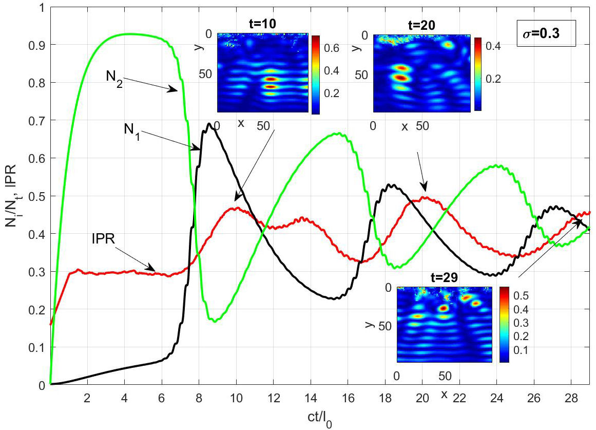
FIGURE 4 (Color online) Dynamics of laser levels populations N 1, N 2 and IPR for σ = 0.3. The insets show that the peaks of IPR shown in Fig. 3b) correspond to the 3D localized field modes in the times where the IPR ∼ 0.5, these times are t = 10,20 and 29.
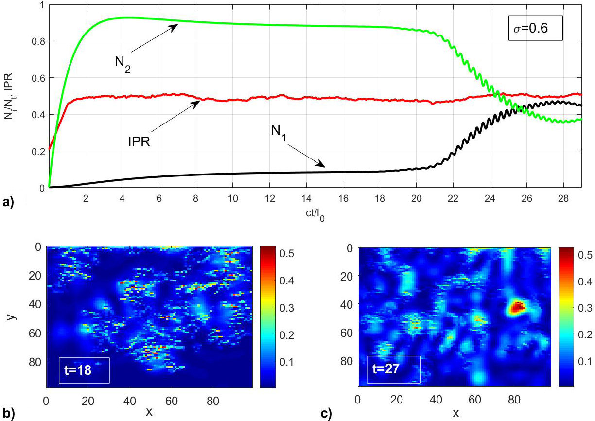
FIGURE 5 (Color online) Numerical simulations made for system cubic network of size L = 100 for σ r = 0.6. a) Average of the IPR calculation as a function of time, (red line). Densities of the lasing levels N 1, and N 2, black and green line respectively. b) Distribution of the |E x | field at time t =18, the spot color boxes show the field in the position of the emitters. c) Distribution of the |E x | field at time t =27, the point around x =85, y =40 exhibits the localized field amplitude.

FIGURE 6 (Color online) Amplitude of the field |E x |, generated by the emitters incorporated in the percolating cluster at σ =0.6. Arrow A shows one of the localized field mode in the 3D cube. b) Same as in a), but with a more detailed view, where one of the localized modes indicated by the symbol A is displayed in part of 3D cube.
Figure 1 shows the dynamics of levels N 1 and N 2, as well as the energy flow I x in the x direction, when σ = 0.04. After an initial excitation time a large number of emitters are synchronized to contribute to the stimulated radiation, this is observed in the I x curve (blue line), which shows some oscillations over time, these oscillations are the result of the inhomogeneity of the structure. We can clearly see that I x has three maxima over time, specifically at times t = 8,19 and 28.
When an excitation is applied, this causes the atoms initially in the lower energy level (N 1) to begin stimulated transitions or “jumps” up to the higher energy level, so we can observe that the first oscillation of the N 1 level ( black curve) is ascending near time t = 6. At the same time, the same applied excitation will also cause any atom initially at the higher energy level (N 2) to start making stimulated transitions and their energy jump down at a rate that is proportional to the intensity of the applied signal, multiplied by the number of atoms at the initial level (that is, higher). We can observe the above in the initial behavior of N 2.
At the intersection of both levels (N 1 and N 2) the maximum amount of energy emerges in the percolation cluster, this is why at t = 8 we observe the greatest amplitude for I x . The same goes for times t = 18 and 28, but with smaller amplitudes.
Figure 1b) shows the dynamics of the IPR as a function of time, we can see two maxima in the IPR, labeled as M 1 at t = 10.5 and M 2 at t = 22. In a neighborhood of M 1 we found a dominant mode with localized field amplitude for a time t = 10. However, in the vicinity of M 2 there has not been enough accumulated energy to obtain a localized field, this is because at that point the IPR ∼ 0.38, which is not sufficient to achieve the effects of localization in the environment, as explained in Sec. 2.
Figure 2 shows the dynamics of N 1, N 2 and the IPR as a function of time for σ = 0.1. We can observe that the IPR reaches its maximum values with the possibility of finding a field localized at times t = 10, 21 and 29; these maxima of the IPR are associated with the decay of the N 2 level. By conservation of energy, the radiation must flow somewhere, and this is reflected in the elevation of the IPR values. Above the graphic of the IPR (in red), we can observe the modes localized in the vicinity of the aforementioned times; these, modes are shown in Fig. 3.
Figure 3 shows the distribution of the |E x | field in some times for the results shown in Fig. 2. In Fig. 3, we can see some circles with a field width localized for different times. Here z represents one of the 3D system planes for a better viewing. We want to note that there is no single time for which we can find a localized field, but in the vicinity of the maximum (IPR) ∼ 0.5, the probability of finding high amplitude modes is very close to one, as we show below.
In Fig. 4, the same as in Fig. 2 is shown, but now σ = 0.3. In this situation, percolation has not yet occurred as in the previous cases. The internal panels show some planes of the 3D system with modes localized in the times where the IPR ∼ 0.5, these times are t = 10,20 and 29.
We want to compare what happens in the sample with incorporated nanoemitters once the percolation has occurred. This situation is shown in Fig. 5, where we have used σ=0.6, a value for which a large cluster is formed that spans the entire network. In Fig. 5a, we can see that there is a longer synchronization time of the laser levels; this is because the number of pores in the system has increased considerably and therefore the volume has increased. Near time t = 28, N 2 reaches its minimum value. It is interesting that the IPR in this situation is a constant value ∼ 0.5, so we would expect that for each time there would be localization of the field. However, in Fig. 5b for a time t = 18, we can observe the positions of the emitters in the sample, and the cooresponding amplitude of the field E x without presenting a localized field. On the other hand, for a time t = 27, after the laser generation has occurred, we observe some mode in the position x = 80, y = 40 (Fig. 5c) with localized field amplitude, other modes appear in the sample but with less amplitude. We can conclude that in order to obtain a field localized at different times, it is necessary and sufficient that the IPR reaches maximum values of approximately 0.5 , and the laser generation occurs in the percolation cluster.
Figure 6 shows the isosurface of the amplitude of the E x 3D field. In this case the field is generated by the emitters incorporated in the percolation system with σ = 0.6. Figure 6a clearly shows some inclusions in blue color occupying different parts of the sample. Figure 6b shows a detailed view of Fig. 6a. We can see that the localized field structure is localized beyond the source area (indicated by the symbol A), whose shape is normally ellipsoidal, coinciding with the characteristic property of finding closed cycles in the optical localization.
One drawback of our proposed method is based on the huge quantity of computational resources needed to work 3D problems. To overcome these limitations, different approaches such as solving the wave equation in the frequency domain could be used, see [37].
4. Conclusions
We have investigated the structure of the optical field radiated by the disordered nano-emitters randomly incorporated in three-dimensional cluster of a percolation material. Our numerical studies shown that the temporal variations of the inverse participation ratio allow analyzing the extended and localized field structures over a long time range. The properties of IPR and the dynamics of the lasing emitters allow to find the characteristic time scales when the localization of the field in a general three-dimensional disordered system occurs.
Studied conditions are considered for a general case and thus, are independent of the occurrence/absence of the percolation in system. Due to this study, one can evaluate the times in which the localized modes of maximum amplitude are recovered in the 3D system. The combination of localization and random lasing has practical consequences because every individual random-laser source would give a unique emission spectrum defined by the specific localized modes in each sample. Such modes can be used as resonators to add functionality to photonic components. The studied effect opens new perspectives to control the optical fields localization in modern optical nano-technologies.

