1.Introduction

Balthazar Van der Pol (1899-1959) was a Dutch electrical engineer. During the 1920s and 1930s, he worked towards the development of radio and vacuum tube technology. Accordingly, he developed an interesting mathematical model, now known as the Van der Pol equation, to describe stable oscillations, called limit cycles, in electrical circuits that employ vacuum tubes. When these circuits are driven near the limit cycle, they become entrained, i.e., the driving signal pulls the current along with it. Van der Pol and his colleague, Van der Mark, reported that at certain drive frequencies, an irregular noise was heard, which was later found to be the result of deterministic chaos ¹. Recently, Van der Pol equation has been used in both physical and biological sciences, among many other areas. For instance, Fitzhugh ² and Nagumo ³ used the equation on a planar field to model the action potential of neurons. The equation was also employed in seismology to model the plates in a geological fault ⁴. Also, Shuto ⁵ has used this equation to study cavity formation modeling of fiber fuse in single-mode optical fibers.

An important research area for nonlinear optics is optical phase conjugation (OPC). One possible way to obtain OPC is through Four-Wave Mixing (FWM), where a link is established between two coherent optical beams propagating in opposite directions with reversed wavefronts and identical transverse amplitude distributions ⁶. In addition to FWM, there are many further approaches to produce the backward PC beam; another approach is based on a variety of backward stimulated scattering processes such as Brillouin (SBS), Raman (SRS) or Kerr ^7,8,9, of which the last one is based on one-photon or multi-photon pumped backward stimulated emission-processes. The basic characteristic of a pair of PC beams is that the aberration influence imposed on the forward beam propagating through an inhomogeneous or disturbing medium can be automatically removed for the backward beam passing through the same medium.

In the present work, the dynamical behavior of a beam that spatially behaves according to a Van der Pol map, here called a Van der Pol beam, within a ring phase-conjugated cavity is modeled. As shown, the behavior of a beam may be obtained by making an arbitrary well-defined chaotic map ^10,11,12. Particularly, the Henón ¹⁴, Bogdanov ¹⁵, Ikeda ¹⁶, Duffing ^17,18, Standard ¹⁹ and Tinkerbell maps ^20,21 were employed, among others. Here, for the first time to the best of our knowledge, a PC laser ring cavity is designed to produce Van del Pol beams within certain well-defined parameters. The structure of this article is as follows. In Sec. 2, a derivation of the Van der Pol map is sketched following Refs. ^22,23,24. In Sec. 3, the ABCD matrix formalism is used to describe an optical cavity; as known, this formalism is commonly used in paraxial optics ²⁵, allowing the representation of each optical component as a 2×2 matrix. Furthermore, the two-dimensional map converted into a theoretical matrix system enables us to reproduce a complex dynamical behavior of the Van der Pol map within a PC ring cavity. As follows, in Subsecs. 3.1 and 3.2, a general case of the Van der Pol beams is approximately obtained. In Sec. 4, the numerically obtained results are discussed. Finally, in Sec. 5, our main conclusions are given.

2.Van der Pol map

There is a large list of bi-dimensional maps (see ²⁶, for example), and one of them is the Van der Pol map. It is known that many oscillating circuits can be modeled by a second-order differential equation of the form

This differential equation is known as Lienard’s equation ²⁷. Clearly, it may be interpreted as the equation of motion for a unit mass object subject to a nonlinear damping force and a nonlinear restoring force. Lienard’s equation may also be written in the phase plane as

where under appropriate f(x) and g(x), the system has a unique, stable limit cycle ^23,28,29. This is explained in the following theorem.

Theorem 2.1 (Lienard’s theorem). Suppose that f(x) and g(x) satisfy the following conditions:

Then, the system (2.2) has a unique, stable limit cycle surrounding the origin at the phase plane.

The Van der Pol oscillator is a model that was originally developed to describe the behavior of nonlinear vacuum tube circuits. In a self-maintained electrical RLC circuit, where the capacitor C is initially charged, and R is a non-linear resistance, the tension is defined as ²⁵

where

and

with i₀ and R₀ being the current and normalized resistance, respectively. Substituting Eqs. (4), (5) and (6) in (3), we have

Differentiating Eq. (7) with respect to τ,

introducing

and

where ωe=1/LC, we obtain

and

By substituting Eqs. (11) and (12) in Eq. (8) yields

By setting μ=R0C/L, Eq. (13) can be transformed to the following form:

Since this differential equation is isomorphic to Lienard’s Eq. (1), it satisfies Eq. (1). In this sense, the Van der Pol equation obeys Lienard’s transformation:

and

There are many methods to numerically solve non-linear differential equations, such as the Runge-Kutta or Euler discretization methods. Using the last one, we rewrite the above system as ³⁰

and

where y_n and θn are the scalar variables, h is a discretization step, and μ is the map parameter. This system may be written in the matrix form of a Van der Pol map as

with elements

B=h, (20b)

C=-h, (20c)

and

Dh,μ,yn=1+hμ1-yn2. (20d)

3.ABCD optic matrix of the Van der Pol map in a ring PC cavity

It is known that an optical system may be described by a 2 x 2 matrix in the paraxial optics approximation. Assuming cylindrical symmetry around the optical axis and defining a z optical axis, both the perpendicular distance of any ray to the optical axis and its angle to the same axis are given by y(z) and θ(z) when the ray undergoes a transformation as it travels through an optical system represented by the matrix [A,B,C,D]; the resultant values of y and θ are given by

For an optical system, it is possible to obtain the total transformation matrix through the product of all the matrices that describe the elements of the optical system. In the considered ring cavity shown in Fig. 1, there are two plane mirrors [M] and an ideal PC mirror [PM], separated by a distance d. The matrices which represent these two elements are: identity matrix

1001

for mirrors [M],

100-1

for the ideal PC mirror [M],

c1d01

for the propagation through distance d, and

cabcd

for the chaos generating device that is located between the two plane mirrors [M] at a distance d/2.

Figure 1 Schematic diagram of the phase conjugated ring resonator studied. There are two plane mirrors [M] and an ideal Phase Conjugated Mirror [PM], separated by a distance d, and chaos generating device represented by matrix [a; b; c; e]. 

For this system, the total transformation matrix [A,B,C,D] for a completed round trip is:

The above one round trip total transformation matrix is:

As seen in the matrix in Eq. (23), each of the elements depends on the elements of the map generating matrix device [a,b,c,e]. However, if one does want a specific map to describe a beam within an optical cavity, then each trip of the beam described by ( yn,θn) ought to be an iteration of the map. Then, the matrix [A,B,C,D] of the map Eq. (19) must be equated to the cavity matrix in Eq. (23), in order to generate a dynamic map for ( yn,θn) in accordance with the Van der Pol map.

Notice that result Eq. (23) is only valid for a small 𝑏, i.e., b ≈ 0. This is because before and after the chaos generating element [a,b,c,e], we have a propagation distance of d/2. For a general case, we have:

Then, the complete round trip transformation matrix in the general case is

Thus, matrix (23) describes a simplified ideal case, whereas matrix (25) describes a general case, more complex and realistic.

4.Numerical experiment

The dynamic behavior of the PC cavity in phase space was studied through numerical iteration of the obtained matrices describing the system. In order to find valid trajectories, there are considerations that have to be taken into account. The phase plane values for y _n and θ_n must be real numbers at every iteration; diverging trajectories are only mathematical possibilities, since they cannot be related to any physical sense. Also, the b _n intracavity element from the matrices must be greater than zero and smaller than the mirror separation distance d in the cavity at every iteration. These conditions ensure that the trajectories are on the real phase plane and within a stable trajectory, given that the b_n element is related to the total distance traveled by the Van der Pol beam within the cavity.

The iterations were carried out for different values of μ and h. As it was stated, μ represents a non-linearity term of the Van der Pol map; we will explore values for this parameter around zero. The stability and chaos of the Van der Pol map in terms of the parameter μ and step h are presented in the phase diagrams (Figs. 2 and 4). Value h was varied for positive numbers till zero, while μ was taken within a range of -1.5 < μ < 1.5. For the 1 < h < 0 range, there are stable trajectories, and the values of b_n are positive and within the limit of the mirror distance. In the figures below, the values of μ and h are not unique, and there are other allowed combinations. Figure 2 shows the phase-space plots corresponding to different values of parameters μ and h. For example, for parameters μ = -1.5 and h = 0.0250, there are no stable states (Fig. 2a)), whereas for μ = -0.5 and h = 0.1196, there is a stable fixed point (Fig. 2(b)). In Figs. 2(c-f), we present the cases of the stable limit cycle.

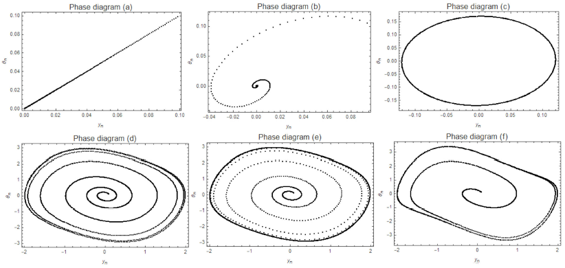
Figure 2 Phase space (yn; θ _n ) trajectories for parameters a) μ = 1:5 h = 0:0250, b) μ = -0:5 h = 0:1196, c) μ = 0 h = 0:0923, d) μ = 0:2 h = 0:0282, e) μ = 0:2 h = 0:0846, f) μ = 0:5 h = 0:0250. In all cases d = 1. 

Figure 3 Time series of intracavity element b _n for 2000 iterations for parameters a) μ = -1:5 h = 0:0250, b) μ = -0:5 h = 0:1196, c) μ = 0 h = 0:0923, d) μ = 0:2 h = 0:0282, e) μ = 0:2 h = 0:0846, f) μ = 0:5 h = 0:0250. In all cases d = 1. 

Figure 4 Phase space (y _n ; θ _n ) for the Van der Pol Map general case for constants a) μ = 0 and h = 0:1, (b) μ = 0 and h = 0:0001. In all cases d = 1. 

The time series of the matrix element b is presented in Fig. 3. The behavior is quite interesting since different dynamical regimes are observed. The numerical simulations were performed for 2000 iterations for matrix element b of the Van der Pol map generating device for a cavity of unitary length (d = 1) and map parameter close to zero. Figures 3(a-c) show damping transients to a stable equilibrium, while Figs. 3(d-f) show others to a stable periodic orbit. One can see from Figs. 3(d-f) how the optical length of the map generating device varies on each round trip in the periodic form (bistability); this would require for a physical implementation such that the physical length of the device, its refractive index, or a combination of both change in time.

The phase diagrams for the general case are shown in Figs. 4 and 5. The process of selection of ℎ and 𝜇 was the same as stated above. Valid trajectories were difficult to find in this case due to the matrix complexity; however, as it was found for μ = 0 and h near zero, the trajectories are not stable and increase on each round trip. Notwithstanding the behavior observed in Figs. 5a) and 5b) for matrix element b, after a few iterations, the device’s optical thickness remains constant, which should make it easier to achieve a physical implementation of this device. Note that in Fig. 5b), the thickness is near zero, while in Fig. 5a), the thickness is around 0.3.

Figure 5 Computer calculation of the magnitude of matrix element b _n of the Van der Pol Map generating device for a resonator with d = 1 and Van der Pol parameters a) μ = 0 and h = 0:1, (b) μ = 0 and h = 0:0001, for 3000 round trips. 

5.Conclusions

In this paper, a matrix transformation over the Van der Pol map has been proposed to obtain an intracavity element that can yield the same rich, dynamical behavior within a ring phase-conjugated ring cavity. We began our study by obtaining the Van der Pol map through the use of the Euler method for discretization; then, we introduced the paraxial matrix analysis (or ABCD propagation law), which was done in order to simplify the analysis, enabling us to express this system as a simple dynamical matrix Equation (3.1). The so-called “Van der Pol beams” (beams that are produced within an optical cavity undergoing Van der Pol map dynamics) were obtained, and they were studied assuming a negligible thickness of the intracavity element, as well as the general case. Numerical calculations were carried out to obtain, within the parameter space, combinations of parameters that yield stable trajectories; this is not an easy task, as the stability of the trajectories is also dependent on the initial value (y _n ), and therefore, the trajectories often do not have physical meaning. It is important to remark that we analyzed valid intervals of the system parameters (μ,h, and d).

The range of the μ parameter was selected based on the meaning of the Van der Pol equation, which determines the non-linearity term. However, if one takes values of μ greater than 1.5 or lower than -1.5 for any values of h, the trajectories, and the intracavity element have no physical meaning. Then, for values of μ within this range, we took different values for h and obtained different results with no physical meaning, except for those varying within the 1 < h < 0 range.

In a simple case of “Van der Pol Beams”, we have found trajectories which began in one value and finished around another (refer to Figs. 2a) and 2b)); these types of trajectories allow the intracavity element 𝑏 𝑛 to reach one value to be stable (refer to Figs. 3a) and 3b)). However, we have also found stable trajectories (Figs. 2d), 2e) and 2f)), which translates into bistability of the intracavity element, and the optical length of the map generating device varies on each round trip in a periodic form; see Figs. 3d), 3e) and 3f). In Fig. 2(c), the trajectory is completely stable, and the parameter of the non-linearity term is zero; this allows the element b_n to remain constant along with the iterations, which allows for easy implementation of the device.

Next, we moved on to the general case, where the thickness of the intracavity element is greater than zero. Even though the trajectory is not stable because of the increasing values of (y_n, θ_n) (See Fig. 4), the element b_n reaches one value (See Fig. 5), making it possible for the optical length to be constant on each round trip.

Based on the behavior observed, we conclude that the matrix transformation used was successful in generating a dynamic system that preserves the main structures found in the Van der Pol map. The practical implementation of an intracavity element is a complex technical challenge far beyond the aim of this work.