1.Introduction

Chaos, bifurcations, and Lyapunov exponent are longestablished mathematical problems that continue to generate much attention. Chaotic systems can be found in physics (e.g., the Lorentz actuator), in finance, in biology, or electrical circuits (e.g., Chua’s electrical circuits); for other fields where chaotic behaviors can be found, see Refs. ^2,3,7,8,13. In 1993, Chua et al. introduced the idea of modeling electrical circuits through chaotic systems ², and Chua’s electrical circuits have found interest in the literature. In chaotic systems, three concepts are fundamental. The first is the stability analysis of the equilibrium points. The stability consists of studying how a solution converges asymptotically around an equilibrium point, taking into account the initial condition. Note that chaotic systems are very sensitive to the initial conditions, where the behavior can easily change. In general, chaotic systems are described utilizing many parameters, and it is also crucial to analyze the chaotic behavior generated by the changes in the values of these parameters, the so-called bifurcations. In other words, in bifurcations, we analyze the impact of the changes in the parameters of the model on the behavior of the chaotic system. Another concept is the Lyapunov exponent, which is used to characterize the existence of chaos or not; the determination of this number is done numerically in fractional cases. Recent years fractional calculus have ^17,28 emerged and attracted many authors. This new field finds much application in the following areas: physics ^11,16,29,31, mechanics, biology ³⁰, mathematical physics, electrical circuits , economics, modeling fluids ^{21 25} and many others^12,24,27. Following this direction, the Chua’s system is remodeled in this paper using the Caputo-Liouville fractional derivative.

There exist many papers that address chaotic models. The literature is long, but we give a brief presentation. In ¹, Cheng et al. investigate the synchronization of the fractional Chua’s chaotic model. In ², Chua et al. introduce an electrical circuit chaotic model and study the synchronization of this proposed model as well. Note that all investigations on Chua’s electrical circuits come from this original paper. In ³, Abdelouahab et al. propose a bifurcation analysis of the fractional-order simple chaotic electrical circuit. In Ref.⁴ Maksoud et al. present the implementation of fractional Chua’s chaotic system by using Grunwald-Letnikov’s derivative. In ⁵, Hartley et al. present the fractional Chua’s electrical circuit using the Riemann-Liouville derivative. The authors, in their investigation, analyze the impact of the fractional-order derivative into Chua’s electrical circuit. In ⁶, Wang et al. investigate on generating multi-scroll Chua’s attractors using the simplified piecewise-linear Chua’s diode. In ^{7 13}, Petras presents the control problem in the context of the fractional Chua’s electrical circuit. In ⁸, the author uses the Atangana-Baleanu derivative for modeling the fractional Chua’s electrical circuit.

The objective of this paper is to revisit the Chua’s electrical circuit described by fractional-order derivative. The motivations for this use are explained in the next section. The model is new. Therefore the stability analysis of the equilibrium points has been studied. The second step will be to analyze the evolution of Chua’s chaotic system when the different parameters of the model have been modified. We mainly use the bifurcation notion to do this investigation. The other point in the research is the characterization of chaos. In other words, we use the determination of the Lyapunov exponent to characterize the existence of the chaos for a particular order of the fractional-order derivative. Note that due to the form of the fractional Chua’s electrical circuit, we decompose the fractional differential equations in three different sub-systems. The research of adaptative control will close this present work.

2. Basic definitions of fractional operators

The fractional derivative is used in this paper for modeling Chua’s electrical circuit. The motivations for such use are described in the next section. In this section, we remind the fractional derivatives used in this paper. We recall, respectively, the fractional integral, the Riemann-Liouville derivative, and the Caputo-Liouville fractional derivative. We have the following definitions.

Definition 1 ^17,28We represent the Riemann-Liouville integral of the functionx:[0,+∞]→Ras the following form

under Γ(…) represents the Gamma function and with the order α obeying the condition that a > 0.

Definition 2 ^17,28 We represent the Riemann-Liouville derivative of the function x:[0,+∞]→R, of order 𝛼 in the following form

with t > 0 , the order α∈0,1 and Γ(…) denotes the Gamma function.

Definition 3. ^17,28 We symbolize the Caputo-Liouville fractional derivative of the function x:[0,+∞]→R, of order 𝛼 in the following relationship

with the conditions t > 0 , the order α∈0,1 and Γ(…) represents the gamma Euler function.

There exist many other types of fractional-order derivatives. In recent years, fractional derivatives with non-singularities have attracted a lot of attention. The definitions of these derivatives can be found in Refs. ^9,10.

3.Presentation of the new fractional Chua’s electrical circuit model

In this section, we present the fractional-order Chua’s electrical circuit represented by Caputo-Liouville fractional derivative. The Chua’s model is an electrical circuit including the resistor R, the inductor L, two capacitors C₁ and C₂, and a nonlinear resistor N_R. The classical model can be represented by the following differential equations ²

where the function g can be represented as the following form

where VC1 is the voltage across the capacitor C₁, VC2 is the voltage across the capacitor C₂, I is the current through the inductance, G_a and G_b are the slopes, and ±B_p denote the breakpoints. Under the following change of variables:

and

Chua’s model can be rewritten as

In general, the fractional-order Chua’s electrical circuit can be obtained by replacing the integer-order derivative with non-integer order derivative; the reasons for this replacement are given next. We have

with the initial conditions represented by the following relationships

and where the function F(x) is defined as follow,

Owing to the fact that Chua’s electrical circuit -in the context of fractional order derivatives- has not been much exploited, it is our motivation to extend Chua’s model ot the non-integer-order derivative case. This paper will be interested in the Chua’s electrical circuit using the Caputo-Liouville fractional derivative. Another motivation in this paper is to see what happens with Chua’s circuit when the non-integer-order derivative replaces the integer-order derivative. The question related to the use of the fractional-order derivative comes from the Leibniz question, where one tries to obtain the value of

when a = 0.5. This question is reasonable because when a = 1, we recover the integer-order derivative. In fractional calculus, the intuition dictates that many phenomena can be described by models using fractional-order derivatives. Many arguments support these reasons. First, we notice all models in real-word problems contain error terms in measuring the real data; for example, in econometric models, where all models are linear differential equations with error terms. Other situations, like the data collected for the revenue and the consumption do not follow exact linear differential relationships because of the amount of existing error terms. For the deterministic differential equations, we notice the one of the solutions do not follow the behaviors obtained with real data. It is because of these reasons that the stochastic representations of differential equations are introduced. For short, many of the phenomena that is commonly represented with integer-order derivatives, are not being described adequately at all times. To take into account all these errors, the fractional-order derivatives are proposed for solving real-world modeling problems.

4.Numerical investigation of the fractional model

In this section, we describe and apply the numerical scheme considered in this paper. The numerical scheme is motivated by the fact the analytical solution of the Chua’s electrical circuit is quasi-impossible. The homotopy methods can be used; the problem will be, after how many iterations the solutions will converge. We use the numerical scheme of the Riemann-Liouville fractional integral. Note that the following representations give the solutions of the fractional Chua’s electrical circuit

where the functions ς, ξ and ζ come from the chua’s electrical model considered in this paper, we have the following

At the point t_n the discretization should be represented in the following forms

Using the grid t_n = nh, where h represents a constant step-size, the scheme of the fractional integral operators are given by

where the parameter is given by dn-j=(n-j+1α-n-jα)/1Γ1+α. We utilize now the first-order interpolant polynomial of the functions ςτ,x(τ), ξτ,y(τ) and ζτ,z(τ) expressed as the following forms

Taking into account Eqs. (31)-(33), the numerical discretizations of the fractional integrals are represented by the following expressions

where the parameters in the above equations are represented in the following expressions

and when the indices describe the set n = 1,2,…, the previous parameters can be expressed as the following form

Finally, as numerical schemes for Chua’s electrical model in the context of fractional order derivative, we have the following representations

Where

We finish this section by recalling some explanations concerning the stability and the convergence of the proposed numerical schemes. We consider that x(tn),y(tn) and z(tn) the numerical approximations of the Chua’s electrical model and x_n, y_n and z_n the exact solutions of the same model. We can write the residual functions as the following forms

The convergence of the used numerical scheme comes from the fact h converge to 0. The stability of the numerical schemes in this paper is obtained by the fact the functions ς, ξ and ζ are Lipschitz continuous.

5.Stability analysis of the equilibrium points

In this section, we study the stability of the equilibrium points of the fractional Chua’s electrical circuit. The main idea is to decompose the fractional system into three cases. In the first case, we suppose ∈(-∞,-1), where f(x)=bx-a-b. In this case, fractional Chua’s electrical circuit is given by

As supposed by Chua’s, we set the parameters to d = 10, c = 14.87, a = -1.27, and b = -0.68. The equilibrium points of the fractional equations represented in Eqs. (48)-(50) are given by

It is straightforward to obtain the Jacobian matrix at the equilibrium point (x*, y*, z*); we get the following relationship

Considering the values of the parameters of the fractional Chua’s model, the characteristic polynomial of the Jacobian matrix is given by

The eigenvalues of the are given by the λ₁ = -4.6597, λ2 = 0.2298+3.1873i , and λ3 = 0.2298-3.1673i. We note that argλ1=π>απ/2 for all α∈(0,1), argλ2=43π/90>απ/2 when α<0.95, and argλ3=137π/90>απ/2 for all α∈(0,1). Thus, we conclude the equilibrium point (x*, y*, z*) is locally asymptotically stable when the order satisfies α<0.95. If not, the equilibrium point is unstable.

For the second case, we suppose x∈-1,1, where f(x) = ax, where the fractional Chua’s electrical circuit is given by

We consider the values d = 10, c = 14.87, a = -1.27, and b = -0.68. The equilibrium point of the fractional equation represented in Eqs. (54)-(56) is given by

The Jacobian matrix at the equilibrium point (0,0,0) is

Considering the values of the parameters of the fractional model, the characteristic polynomial of the Jacobian matrix is now

Direct computation using Matlab shows that the eigenvalues of P(λ) are given by the λ1=3.8477 λ2=-1.0739+3.0465i and λ3=-1.0739-3.0465i. We note that argλ1=0<απ/2. Thus, it is concluded that the equilibrium point (0,0,0) is not stable.

In the last case, we suppose x∈[1,+∞] where f(x) = bx + (a - b) , in this case the fractional Chua’s electrical circuit is given by

Following the work of Chua, we consider d = 10, c = 14.87, a = -1.27, and b = -0.68. The equilibrium point of the fractional Eqs. (60)-(62) is given by

The rest of the procedure is identical as in the first case. It is straightforward to see that the Jacobian matrix at the equilibrium point is given by the following relationship

Considering the values of the parameters of the fractional model, the characteristic polynomial of the Jacobian matrix is given after calculation by the following form

The eigenvalues are given by λ1=-4.6597, λ2=0.2298+3.1873i and λ3=0.2298-3.1873i. We note that argλ1=π>απ/2 for all α∈(0,1), argλ2=43π/90>απ/2 when a < 0.95, and argλ3=137π/90>απ/2 for all α∈(0,1). Thus, we conclude the equilibrium point is locally stable when the order satisfies the condition a < 0.95. If not, then the equilibrium point is unstable.

Finally, we can observe the trivial equilibrium point is not stable, but the two non-trivial equilibrium points are locally stable under the condition the fractional-order derivative does not exceed 0.95.

6.Graphical support of the numerical scheme

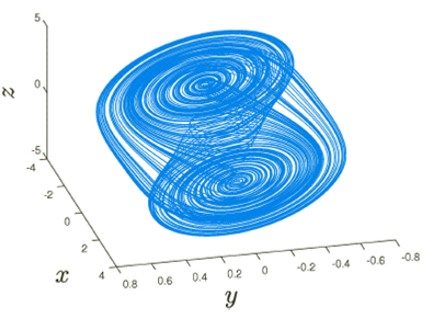
In this section, we study the chaotic behaviors of the fractional Chua’s electrical circuit. We represent the solutions graphically by using the numerical discretizations described in the previous section. We also analyze the impact of the different parameters using the bifurcation concept. Note that a bifurcation is a tool used to analyze the sensitivity of the fractional differential equation due to the variation of one of its parameters. For the rest of the paper, we suppose the following initial condition: x(0) = -0.68, y(0) = 0 and z(0) = 0.68. The parameters of the model are d = 10, c = 14.87, a = 1.27 and b = - 0.68 and we consider the order a = 0.95.

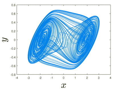
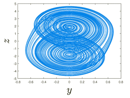
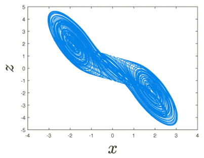
Figure 1 focuses on the dynamics of the fractional Chua’s electrical circuit in the axis 𝑥-axis, 𝑦-axis and𝑧-axis. Figure 2 highlights the dynamics of the fractional Chua’s electrical circuit on the 𝑥-axis, and 𝑦-axis. Figure 3 describes the dynamics of the fractional Chua’s electrical circuit on the 𝑦-axis, and 𝑧-axis. Figure 4 depicts the dynamics of the fractional Chua’s electrical circuit on the 𝑥-axis, and 𝑧-axis.

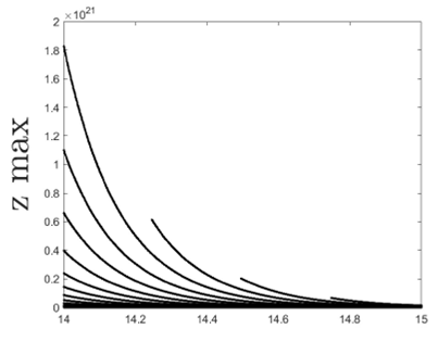
Let us now analyze the impact of the parameter d∈(9,11) on Chua’s electrical circuit. The other parameters of the model are supposed constant and do not vary. In Fig. 5, we depict the bifurcation diagram with the variation of the parameter d. Let us explain the dynamics represented in Fig. 5 and give its physical meaning. According to reference ³, when the parameter d∈(9,10.5), it corresponds to the asymptotic stability of the trivial equilibrium point, the Chua’s system exhibits chaotic behaviors when d exceeds 10.5.

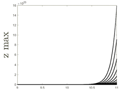
We continue by analyzing the impact of the parameter c∈(14,15) on Chua’s electrical circuit. The other parameters of the model are assumed to be constant. In Fig. 6, we depict the bifurcation diagram with the variation of the parameter c. Let us explain the dynamics represented in Fig. 6 and to give its physical meaning. According to Ref. ³, when the parameter c∈(14,14.6), Chua’s system exhibits chaotic behaviors and when c exceeds 14.6, which corresponds to the asymptotic stability of the trivial equilibrium point, confirming the previous analysis related to the stability and the chaotic behavior observed in Figs. 1-4.

We finish by proposing the Lyapunov exponent of the fractional Chua’s electrical circuit. The importance of the Lyapunov exponent is to detect the presence of chaotic behaviors. There exist some methods proposed in the literature for the detection of the chaos in the fractional context like the method proposed in Ref. ³³ based on the semi-analyticalsolution, and the Lyapunov exponent base on the numerical scheme and the Jacobian matrix, as described in our context ³². As for the detection of the presence of chaotic dynamics, it is said that when the maximal value of the Lyapunov exponent is large and positive, then chaotic behaviors are taking place. As previously discussed in the bifurcation section, we fix a = 0.95, and d = 10, c = 14.87, a = -1.27, b = -0.68 and f(x) = ax. The method of the determination of the Lyapunov exponent is described in the context of the fractional calculus in ³². The novelty in the determination of the Lyapunov exponent in our context is that we replace the numerical scheme used in by our numerical scheme, and utilize the Jacobian matrix of Chua’s model. It is also important to mention that the value of the Lyapunov exponent is sensitive to the initial conditions. Here, the initial conditions are x(0) =- 0.68, y(0) = 0 and z(0) = 0.68. Under such initial conditions, the maximal values of the Lyapunov exponent of the fractional Chua’s model when a = 0.95 is obtained at time T = 19.98 and is given by LE = 0.3270. The maximal Lyapunov exponent is positive and large, confirming the existence of high chaotic behavior, as we can observe in Figs. 1-4.

7.Adaptative controls

In this section, we propose an adaptative control under which the driving system and the response system oscillate or go in the same direction. It is essential when the stability analysis of a particular model is not trivial. In the first case, we consider the driving Chua’s model described by

Let the response fractional chaotic Chua’s model given by

where the control input is supposed as follows u=u1,u2,u3. In the first case, the objective will be to give adaptive values to the control inputs. Let the error terms be defined by

Applying the Caputo-Liouville fractional derivative to the error terms we get the following fractional differential equations

We propose the following control u = (0,0,0) and we prove using the Lyapunov function that the fractional differential equation given by Eqs. (73)-(75) is globally asymptotically stable. Let the Lyapunov function defined by

We continue with the linear fractional differential equations. Then the Caputo-Liouville fractional derivative along the trajectories of Eqs. (73)-(75) is represented by the following relationships :

Thus, under the supposed control, and the supposed parameters of the model, we observe Eq. (77) is a negative term; that is, the trivial equilibrium of fractional error system is globally asymptotically stable, which in turn implies that limt→+∞η=limt→+∞y-x =0. Finally, the driving system and the response of the fractional Chua’s electrical circuit go in the same way when the signal control is u = 0.

In the second case, we repeat the same procedure, since not many changes are done in the calculations. We consider the driving Chua’s model described by

Let the response fractional chaotic Chua’s model given by

where the control input u=u1,u2,u3. In the second case, the objective will be to give adaptive values to the control inputs. Let the error terms be defined by

Applying the Caputo-Liouville fractional derivative to the errors terms, we get the following fractional differential equation

We propose the following control u = (0,0,0) and we prove using the Lyapunov function that the fractional differential equation given by Eqs. (85)-(87) is globally asymptotically stable. Let the Lyapunov function defined by :

The rest of the proof is not difficult to perform and we fall on the linear fractional differential equation. Then the Caputo-Liouville fractional derivative along the trajectories of Eqs. (85)-(87) is represented by the following,

Thus, under the chosen control and values of the model parameters, we observe that Eq. (89) is a negative term; that is, the trivial equilibrium of fractional error system is globally asymptoatically stable, which in turn implies that limt→+∞||η||=limt→+∞||y-x||=0. Finally, the driving system and the response of the fractional Chua’s electrical circuit go in the same direction when the signal control is u = 0.

For the last case, a similar procedure to the one before is followed. We consider the driving Chua’s model described by

Let the response fractional chaotic Chua’s model given by

where the control input is supposed as follows u=u1,u2,u3. In the last case, the objective will be to give adaptive values to the control inputs. Let’s the errors term defined by the following terms

Applying the Caputo-Liouville fractional derivative to the error terms we get the following fractional differential equation:

We propose the following control u = (0,0,0) and we prove using the Lyapunov function that the fractional differential equation (97)-(99) is globally asymptotically stable. Let the Lyapunov function be defined by

We continue with the linear fractional differential equation. Then the Caputo-Liouville fractional derivative along the trajectories of Eqs. (97)-(99) is represented by the following relationships ^23,26:

Thus, under the supposed control, and the supposed parameters of the model, we observe Eq. (101) is a negative term, that is the trivial equilibrium of fractional error system is globally asymptotically stable, which in turn implies limt→+∞η=limt→+∞y-x =0. Finally, the driving system and the response of the fractional Chua’s electrical circuit go in the same way when the signal control u = 0.

8.Conclusion

In this paper, we have revisited the fractional Chua’s electrical circuit. The numerical schemes allow us to get the solutions of the proposed model and to analyze the model have been presented. The qualitative properties as the stability analysis of the equilibrium points, the bifurcation diagrams, and the Lyapunov exponent were discussed. The Lyapunov exponent depends on the chosen initial condition and the considered order for the fractional derivative. Note that this factor proves the existence of highly chaotic behavior when the fractional order is used in modeling Chua’s electrical circuit. This paper demonstrates that the fractional-order can also be used for modeling the electrical Chua’s circuit in general.