SciELO - Scientific Electronic Library Online

 
vol.66 número6Stochastic dynamics for epidemics based on a compartmental scheme: An application to the AH1N1 influenza índice de autoresíndice de materiabúsqueda de artículos
Home Pagelista alfabética de revistas  

Servicios Personalizados

Revista

Articulo

Indicadores

Links relacionados

  • No hay artículos similaresSimilares en SciELO

Compartir


Revista mexicana de física

versión impresa ISSN 0035-001X

Rev. mex. fis. vol.66 no.6 México nov./dic. 2020  Epub 31-Ene-2022

https://doi.org/10.31349/revmexfis.66.874 

Research

Other Areas in Physics

Approximate construction of new conservative physical magnitudes through the fractional derivative of polynomial-type functions: A particular case in semiconductors of type AlxGa1-xAs

J. C. Campos-Garcíaa 

M. E. Molinar-Tabaresb 

C. Figueroa-Navarroc 

L. Castro-Arced 

aDepartamento de Ciencias de la Salud, Universidad de Sonora, Blvd. Bordo Nuevo s/n, Antiguo Ejido Providencia, Apdo. Postal 85040, Cd. Obregón Sonora, México. e-mail: julio.campos@unison.mx

bOrganismo de Cuenca del Noroeste, Comisión Nacional del Agua, Hermosillo, Sonora, México. e-mail: martin.molinar@conagua.gob.mx

cDepartamento de Ingeniería Industrial y Sistemas, Universidad de Sonora, Unidad Centro, Hermosillo, Sonora, México. e-mail: cfigueroa@industrial.uson.mx

dDepartamento de Física, Matemática E Ingeniería, Universidad de Sonora, Unidad Sur, Navojoa, Sonora, México. e-mail: lcastro@navojoa.uson.mx


Abstract

The fractional calculus has a very large diversification as it relates to applications from physical interpretations to experimental facts to the modeling of new problems in the natural sciences. Within the framework of a recently published article, we obtained the fractional derivative of the variable concentration x(z), the effective mass of the electron dependent on the position m(z) and the potential energy V(z), produced by the confinement of the electron in a semiconductor of type AlxGa1-xAs, with which we can intuit a possible geometric and physical interpretation. As a consequence, it is proposed the existence of three physical and geometric conservative quantities approximate character, associated with each of these parameters of the semiconductor, which add to the many physical magnitudes that already exist in the literature within the context of fractional variation rates. Likewise, we find that the fractional derivatives of these magnitudes, apart from having a common critical point, manifest self-similar behavior, which could characterize them as a type of fractal associated with the type of semiconductor structures under study.

Keywords: Educative science; fractional derivative; geometric and physical interpretations; semiconductor parameters; fractional continuity equations

PACS: 01.40.E-; 61.82.Fk; 02.30.Mv; 05.45.Df; 02.30.Gp

1.Introduction

For the scientific community, it is known the great number of works related to the application of fractional calculation in the different areas of knowledge 1-10. In parallel, there are efforts that continue with the objective of performing physical and geometric interpretations of both the fractional derivative and the fractional integral, as shown in recent contributions. See for example: 11-14, where are shown geometric and physical interpretations of Volterra-type convolution integrals a relationship between the fractal set of Cantor and the fractional integral, the presentation of the general conformable fractional derivative, along with its physical interpretation, and the geometric interpretation of the tangent line angle of a polynomial with fractional derivative coefficients, respectively.

On the other hand, independently of the existence of diverse physical and geometric interpretations of what the fractional derivative of the function of a physical system represents, it is important to mention that its use in different sciences, as well as natural (physical) sciences, can be said to be endorsed by the formulation of the variational principles of fractional type, which describes with great success the evolution of non-conservative systems, as mentioned in the references 15,16. Likewise, in related literature, we can find several explicit applications of the fractional derivative in natural systems; for example, in 17, a model is proposed to characterize natural shapes such as neutral hydrogen emissions using the concept of a fractional derivative. Also, in 18, it is found that an approximation can be established between the concepts of relativistic kinetic energy and fractional kinetic energy. The heterogeneous semiconductor structures do not escape this multitude of applications of the fractional calculation; for example, in 19-25 just some of them can be found. Thus, taking into account the favorable effect that the fractional derivative can have on the different natural systems, our present contribution consists in the direct application of the framework developed in 14 to find, for the first time, the approximate physical and geometric effect that produces the fractional derivative of the variable the concentration of a dopant, in this case, Aluminum deposited on a substrate, the position-dependent effective mass adopted by the confined electron, and the potential energy that the electron acquires due to the semiconducting medium. It should be mentioned that we use these magnitudes in a recent contribution 26, where we use the structure formed by AlxGa1-xAs as a semiconductor. Bearing this in mind, the second section contains the description of the mathematical formalism. The third section describes the application of such formalism to the semiconductor parameters of the mentioned type and, finally, in the fourth section, a brief description of the obtained results and the consequences inferred by them are made.

2.Description of the formalism

The concept of a fractional derivative is linked to that of the minimum trajectory to go from a point (x1, f(x1)) to a point (x2, f(x2)) in a plane x, f(x), and then to get the Lagrangian of the system. From the classical theory of differential calculus and integral calculus, we can see that for a function f(x), there is an infinite sequence of derivatives and integrals 27

d2f(t)dt2,df(t)dt,f(t),atf(τ)dτ,ataτ1f(τ)dτdτ1, (1)

The fractional calculation tries to interpolate the sequence (1) in such a way that it allows generating any order from an arbitrary order. Several definitions have been proposed for the fractional derivative, among which are those of Riemann-Liouville, Grünwald-Letnikov, Weyl, Caputo, Marchaud, and Riesz. In particular, in the present work, we make use of a definition that is generated from the fractional derivative of Riemann-Liouville:

cDxαfx=1Γ(n-α)ddxn×cxx-τn-α-1fτdτ, (2)

with 0 < α < 1. Integrating by parts and making a change of variable to introduce the definition of the beta function, it can be seen that for a function of the type f(x)=xc, the fractional derivative to f(x) is given by

Dα[xc]=Γ(c+1)Γ(c+1-α)xc-α. (3)

This type of fractional derivative is used in 14, where the result of Dα[xc] is multiplied by the result of the triangular area Afα formed between the tangent line in (x = b,f(x = b)) the distance between the point where the tangent line crosses the axis x and x = b, and the line x = b, which can be visualized better inspecting the Fig. 1. The result of such multiplication is a constant, i.e., Dα[xc]Afαconstant.

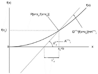
Figure 1 Graphic representation of the geometric and physical elements, described by the mathematical formalism, adopting an order of the fractional derivative of a = 1=2. 

The triangular area Afα of Fig. 1 will be given by

Afα=(λfα[fx=b]2. (4)

The value of λ is solved for the triangular area in the form

tanθfα=mfα. (5)

In such a way that

θfα=tan-1mfα=tan-1{Dα[bc]}=θ0α, (6)

where θ0α is the value of the angle in radians, obtained for a value of α.

On the other hand, from the triangular area we also have that θfα=[fx=b]/[λfα] then λfα=[fx=b]/[tanθα] and substituting θ0α in θα we get λfα=[fx=b]/[tanθ0α].

With this information, the triangular area is expressed as

Afα[f(x=b)]22tanθ0α. (7)

As can be seen, once the values of b and a are determined, both Afα and Dα[bc] can be obtained.

As mentioned in 14, the triangular area Afα represents a physical magnitude by itself, where it is constructed in a geometric form. The same geometrical and physical aspects can be visualized in the fractional variation rate Dα[bc]. These aspects associated with both Afα and Dα[bc] are combined to produce another physical and geometric magnitude, which arises with the multiplication of both, as mentioned in the opening paragraph of this section. This magnitude of invariant character could reflect a type of symmetry, which would manifest depending on the system under study. In the next section, an application of the present formalism is realized.

3.A direct application of the formalism

Using atomic units, the concentration of the semiconductor is given by x(z)=(1.4/L2)z2-(1.4/L)z+0.35. The position dependent effective mass of the electron m(z)=(0.118/L2)z2-(0.118/L)z+0.096 and the potential energy of the electron V(z)=(0.044/L2)z2-(0.044/L)z+0.0110 are polynomial type functions with position dependence z and where L is the size of the crystalline structures. The three magnitudes associated with the semiconductor under study have a similar algebraic structure.

In applying the formalism described in the previous section to x(z), m(z), V(z), respectively, is obtained

Dαx(z)=Dα1.4L2z2-Dα1.4Lz+Dα, (8)

Dαm(z)=Dα0.118L2z2-Dα0.118Lz+Dα0.096 (9)

Dαx(z)=Dα0.044L2z2-Dα0.044Lz+Dα0.0110 (10)

The fractional derivatives (8), (9) y (10) have a graphic structure equivalent to that described by Fig. 1, within the framework of the formalism raised above.

Taking into account the above, the areas Axα=α0, Amα=α0, AVα=α0, are given respectively by

Axα=α0=λxα[xz=z0]2, (11)

Amα=α0=λmα[mz=z0]2, (12)

AVα=α0=λVα[Vz=z0]2, (13)

To solve the areas of (11), (12), and (13), respectively, it is taken into account that

tanθxα=mxα=Dα[xz=z0]θxα=tan-1θxα, (14)

tanθmα=mmα=Dα[mz=z0]θmα=tan-1θmα, (15)

tanθVα=mVα=Dα[Vz=z0]θVα=tan-1θVα, (16)

where mxα, mmα, and mVα are the slopes that touch the curves x(z), m(z), and V(z) forming each of the points P that are reached to be visualized in the previous figures. Likewise, the angles θxα, θmα and θVα are given in radians.

On the other hand, from the same triangles with the areas given by (11), (12), and (13), we also have, respectively that

tanθxα=x(z=z0)λxα, (17)

tanθmα=m(z=z0)λmα, (18)

tanθVα=V(z=z0)λVα. (19)

Therefore, substituting the angles θxα, θmα, and θVα from (14), (15), and (16), in (17), (18), and (19), respectively. With this, it is possible to obtain the lengths of the bases λxα,λmα and λVα of the respective triangles, which finally are replaced in (11), (12), and (13), to obtain the values corresponding to the areas Axα=α0, Amα=α0, and AVα=α0.

Once these areas are obtained, the following physical magnitudes can be constructed

Dα=α0[x(z=z0)]Axα=α0Ξ, (20)

Dα=α0[m(z=z0)]Amα=α0Υ, (21)

Dα=α0[V(z=z0)]AVα=α0Ω, (22)

The Eqs. (20), (21) y (22) represent a type of conservative magnitudes from a geometric and physical point of view. By solving (20), (21), and (22), the constant numerical values associated with the corresponding products are obtained between the fractional derivatives and the respective areas, as can be observed through Tables I, II, and III, where α[0.1000,1.000], with jumps of 0.1000, respectively. Likewise, the value of z = 75 was chosen arbitrarily only to carry out the calculations.

Table I The fractional-order a of the derivative, the fractional derivative of the concentration x(z) evaluated in z = 75, the projected area Axα=α0 for each of the slopes associated with each value of a and the product between the fractional derivative of the concentration in z = 75 and the Axα=α0 respective. The numerical value of L = 100 is adopted for the size of the crystalline structure. 

α =α0 D α= α0[x(z)] Axα=α0 Da=a 0[x(z)] Axα=α0=Ξ]
0.1000 0.0634 0.0604 3.83E-03
0.2000 0.0475 0.0805 3.83E-03
0.3000 0.0366 0.1046 3.83E-03
0.4000 0.0287 0.1332 3.83E-03
0.5000 0.0228 0.1679 3.83E-03
0.6000 0.0182 0.2107 3.83E-03
0.7000 0.0145 0.2647 3.83E-03
0.8000 0.0115 0.3343 3.83E-03
0.9000 0.0090 0.4255 3.83E-03

Table II The fractional-order a of the derivative, the fractional derivative of the effective mass m(z) evaluated in z = 75, the projected area Amα=α0 for each of the slopes associated with each value of a and the product between the fractional derivative of the concentration in z = 75 and the Amα=α0 respective. The numerical value of L = 100 is adopted for the size of the crystalline structure. 

α =α0 D α= α0[m(z)] Amα=α0 Da=a 0[m(z)] Amα=α0=Υ
0.1000 0.0634 0.0604 3.83E-03
0.2000 0.0475 0.0805 3.83E-03
0.3000 0.0366 0.1046 3.83E-03
0.4000 0.0287 0.1332 3.83E-03
0.5000 0.0228 0.1679 3.83E-03
0.6000 0.0182 0.2107 3.83E-03
0.7000 0.0145 0.2647 3.83E-03
0.8000 0.0115 0.3343 3.83E-03
0.9000 0.0090 0.4255 3.83E-03

Table III The fractional-order a of the derivative, the fractional derivative of the confining potential V (z) evaluated in z = 75, the projected area AVα=α0 for each of the slopes associated with each value of a and the product between the fractional derivative of the concentration in z = 75 and the AVα=α0 respective. The numerical value of L = 100 is adopted for the size of the crystalline structure. 

α = α0 =α0 [V (z)] AVα=α0 Da=a 0[m(z)] Amα=α0=Ω
0.1000 0.0020 1.9202 3.83E-03
0.2000 0.0015 2.5622 3.83E-03
0.3000 0.0012 3.3274 3.83E-03
0.4000 0.0009 4.2393 3.83E-03
0.5000 0.0007 5.3419 3.83E-03
0.6000 0.0006 6.7037 3.83E-03
0.7000 0.0005 8.4230 3.83E-03
0.8000 0.0004 10.6375 3.83E-03
0.9000 0.0003 13.5397 3.83E-03
1.0000 0.0002 17.4006 3.83E-03

Likewise, the semiconductor concentration function x(z) can be visualized through Fig. 2, where the triangular areas obey the formalism used in this article.

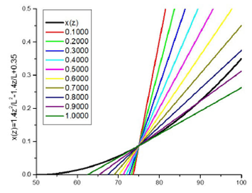
Figure 2 Graphic representation of the geometric and physical elements of the concentration x(z) described by the mathematical formalism adopting an order of the fractional derivative of α ∈ [0.1000; 1.000]. 

Each of the other physical magnitudes (effective mass m(z) and the confining potential V(z)) also have geometric and physical elements, which manifest themselves analogously to the concentration x(z). Once obtained the numeric calculations for the effective mass and the confining potential, it was found that the constant value associated with each of these magnitudes was the same, i.e., it is found that Ξ=Υ=Ω=3.83×10⁻³, which reflects intuitively the

the possibility of new symmetries associated with the semiconductor system. Interestingly, the numerical coincidence of these three new invariant magnitudes could indicate that the semiconductor system has a certain self-similarity, which allows us to characterize it as a structure of fractal type.

Likewise, as we mentioned in 26, there is a visible relationship between x(z), m(z) and V(z), which we can express as x(z)=31.818V(z), m(z)=0.0665+2.681V(z). This relationship allows us to draw some conclusions about the relationship between these semiconductor parameters and the quantum formalism that describes them, that is if we take into account that the Hamiltonian we studied in 26 was independent of time, from there it was. You can see that it

is a linked potential. Such characteristic allows us to infer that (22) is continuous everywhere, as shown in 28. The fractional continuity of (22) is verified because the z coordinate of the semiconductor crystal structure does not have a discrete value spectrum. Likewise, such a continuity equation is a restriction to the wave function of the confined electron, as mentioned in 28. Now, as we already mentioned, the concentration and the mass effectively show a clear relationship with potential, and that relationship allows us to infer that the continuity Eqs. (20) and (21) have an interpretation similar to the continuity (22) of the potential, which is grounded since xz[0,0.35], mz[0.0665,0.0960] and Vz[0,2.75×10-3]. Some fact that results interesting can be seen in the numerical calculation shown in the Tables I, II, and III, where it is observed that the continuity equations are verified even though the order of the derivative α →1.

On the other hand, from these continuity equations, it can be seen that, inside the semiconductor, a fractional area is defined when 0.1000α<1.0000 and only when α = 1, such area is transformed into one of integer degree. So, the areas defined by the respective continuity equations are defined by an inverse relationship with the rates of fractional variation respective. This information could be telling us that there is an area Aα inside the semiconductor, where α may be indicating the degree of irregularity it may have, which is quite possible and real, at least from an intuitive point of view. To go a little deeper into what was mentioned in the previous paragraph. Let us start remembering how in 29, it is mentioned that a semiconductor can be deposited on a substrate, varying its concentration in one direction particular growth, which in turn will cause an effective mass of the electron that will be dependent on its position within the crystal structure. As you can see, the fact of depositing a semiconductor in a substrate in one direction, involves an interaction between a quantity of semiconductor through an area unit, that is, there is a correspondence between a rate of change of concentration Dα=1[xz] and the cross-sectional area Aα=1 where such rate of increase is happening. On the other hand, to guarantee compliance with the energy conservation, we must take into account that the substrate has negligible losses of the semiconductor and whose correspondence happens through an inverse ratio relationship like Aα=11/Dα=1[xz], of such that this proportionality implies the relation Aα=1=Ξ/Dα=1[xz], whose numerical value can be seen in Table I. Likewise, we can notice that such cross-sectional area Aα=1 obeys the Euclidean standard geometry and is due to an isotropic growth rate of concentration Dα=1[xz]. However, it is very interesting to observe that when α < 1, you have Aα<1=Ξ/Dα<1[xz], that is to say, the same quantity Ξ preserved, only now you have a cross-sectional area obeying the Hausdorff fractional geometry. This means, that the area cross-section Aα<1 has a set of degrees of irregularity, which correspond biunivocally with the set of variation rates with equivalent degrees of irregularity or anisotropy in the z direction, as expressed below:

Dα<1xz0.1000,0.9000  Aα<10.1000, 0.9000 (23)

with 0.1000 jumps. Such an interpretation can be visualized through Fig. 3.

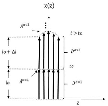
Figure 3 Visualization of the variation rate of x(z), involving an isotropic and anisotropic evolution across cross-sectional areas Euclidean and Hausdorff, respectively. 

From the previous Fig. 3, you can see the visualization of the variation rate of x(z), with dependence on the degree α of the derivative. In the initial time t = t0, the concentration undergoes an isotropic evolution Dα=1[xz] across a Euclidean-like cross-sectional area Aα=1. Later, in times t > t0, the concentration of the semiconductor experiences an anisotropic evolution Dα<1xzα[0.9000,0.1000] through a non-integer dimension Hausdorff cross-sectional area Aα<1α[0.9000,0.1000], where l0 is the initial length that corresponds to the magnitude of Dα=1 and l0+Δl the magnitude of Dα<1 corresponding to α = 0.9000 and so on up to α =0.1000. Therefore, the value of α provides us with information on the degree of anisotropy that the rate of variation of the concentration x(z) and the cross-sectional area involved in the direction in which the concentration, with anisotropy being null when α = 1.000 and anisotropy not null when 0.1000α<1.000. This same interpretative analysis of (20) can be applied to (21) and (22) for the effective mass of the electron and the confining potential, respectively.

4.Critical points in the fractional derivative of x(z), m(z), andV(z)

According to 14, the fractional derivative of polynomial-type functions shows critical points when the base variable and the largest exponent of the polynomial coincide. Then, to visualize some critical points in the fractional derivative of the concentration, effective mass of the electron, and potential energy of the system, it is necessary to pose the corresponding equations of the formalism for each of the magnitudes. However, as all three have the same algebraic structure, we focus only on the concentration x(z), as shown below.

If the fractional derivative of the concentration x(z) of the semiconductor under study is given by

Dαz,β,α=Dα1.4L2zβ-Dα1.4Lzβ-1+Dα0.35zβ-2. (24)

For z = β = 2, we must then have the possibility of finding critical points. We examine this inspection in a next way

Dα(β,β,α)α=α1.4L2Γ(β+1)Γ(β+1-α)ββ-α-1.4LΓβΓβ-αββ-1β-1-α+(0.35)Γ(β-1)Γ(β-1-α)β-2β-2-α=0 (25)

If β = 2, (12) is reduced only to the first two terms

Dα(β,β,α)α=α1.4L2Γ(β+1)Γβ+1-αβ(β-α)-1.4LΓ(β)Γ(β-α)β-1(β-1-α)=0 (26)

Solving the partial derivative (13), we obtain the next equation

1.4×10-422-αΓ(3)-log2+ψ0(3-α)Γ(3-α)-0.01411-αΓ2ψ02-αΓ2-α=0 (27)

which is a general equation for the variable called “critical point α” y where ψ(0) is the Polygamma function.

The solution of (26) provides us with the existence of the critical point α = 0.5, which means that in the interval of α[0.1000,1.000], the fractional derivative of x(z) reaches a maximum in α = 0.5 and from there it starts to decrease until it reaches Dα=1.000[xz]. The equations analogous to (26) can be obtained for m(z), and V(z) and, as a consequence, they will also have the same critical point α = 0.5, maintaining a very parallel behavior in its growth ratios and fractional decrease within the crystalline size of the semiconductor delimited in the present work. Likewise, the numerical solutions of (26), for the intervals of 2<α4, show critical values at the midpoint of the respective interval Δα, while for the intervals of 4<α10, such critical points are displaced from the midpoint in an amount of ≈ 0.1, as can be seen in Table IV.

Table IV Critical points of the fractional derivative of the concentration x(z) evaluated in z = 2, adopting the numerical value of L = 100 for the size of the crystalline structure. 

Δα α
[0.1000; 1.000] 0.5387
[2.1000; 3.000] 2.4956
[3.1000; 4.000] 3.5729
[4.1000; 5.000] 4.6105
[5.1000; 6.000] 5.6352
[6.1000; 7.000] 6.6532
[7.1000; 8.000] 7.6671
[8.1000; 9.000] 8.6784
[9.1000; 10.00] 9.6877

Something interesting that we can also observe, it has to do with the numerical coincidence shown between the critical points shown in Table IV and specific values that involve the Zeta function of Riemann ς(k) given by the next set of equations, respectively,

α1=0.5=k=2-1kςk-1, (28)

αmmk=2ςk-1+k=2-1kςk-1  for m=2,3 (29)

αnnk=2ςk-1+k=2ς2k-1  for n=2,9 (30)

Now, if we take into account that these series that involve the Zeta function of Riemann are produced at the same time by the generating function,

k=2ς(k)yk-1=-ψ(0)(1-y)-γ

being 𝛾 the constant of Euler-Mascheroni, 30 then we could infer that the critical points predicted by (26) can be represented by a generating function like the one shown below

(31)

This coincidence allows us to strengthen the intuitive character that we have towards the self-similar behavior of the fractional derivatives of x(z), m(z), and V(z).

5.Conclusions

In the present work, we carried out an analysis of the fractional derivative applied to the concentration x(z), the effective mass m(z), and the confining potential V(z), which are magnitudes associated with a semiconductor of type AlxGa1-xAs, studied by us in a previous work. We believe that we have achieved, at least approximately, an interpretation possible with the direct application of a formalism that uses the fractional derivative of polynomial-like functions. From the results obtained in the present contribution, we can state that the new constant magnitudes found Ξ, γ, and Ω, show a self-similar process by visualizing the evolution of each of the fractional variation rates over the respective fractional areas (Eqs. (5), (6) and (7)), from an initial fractional-order α i to a final one α i , in the space of the spatial coordinate z. Also, such an evolution could be perceived, in an intuitive way, as the description of “fractional flows through fractional areas”. This result and the intuitive approach with which we approach it leads us to the equation of continuity inspected commonly in university textbooks, which has a similar structure but with the difference that the variational rates are non-fractional variational rates. In the same way, we show, numerically, that the concentration x(z) really behaves as an invariable quantity, verifying the analytical result. The same can be verified for m(z) and V(z). We also find that the fractional derivative of the concentration exhibits a set of critical points, which depend on the interval associated with the fractional order of the derivative.

Finally, it is interesting to reflect on the self-similar behavior in our system, within a given interval for the values of the order of the fractional derivative, knowing that self-similarity is a characteristic feature of a fractal, as mentioned above. This characteristic, together with the property of scale invariance and the symmetry that could be associated with each of the new magnitudes found for the semiconducting system under study, it could be studied more deeply in a future contribution.

It should be noted that the applications and topics reviewed, such as fractional calculation, fractals, and the Zeta function of Riemann, are vitally important for a great diversity of contemporary scientific research.

Acknowledgments

The authors wish to thank the University of Sonora for the infrastructure provided for the preparation of this contribution. We also thank the referee for his important recommendations, which enriched the work considerably.

References

1. A. Bancaud, C. Lavelle, S. Huet, and J. Ellenberg, Nucleic Acids Research 40 (2012) 8783. https://doi.org/10.1093/nar/gks586 [ Links ]

2. F. Wang, Z. Liu, L. Jiao, C. Wang, and H. Guo, Fractals 25 (2017) 1750042. https://doi.org/10.1142/S0218348X17500426 [ Links ]

3. D. Zhang, A. Samal, and J. R. Brandle, International Journal of Pattern Recognition and Artificial Intelligence 21 (2007) 561. https://doi.org/10.1142/S0218001407005090 [ Links ]

4. J. L. Liou, C. M. Tsai, and J. F. Lin, Wear 268 (2010) 431. https://doi.org/10.1016/j.wear.2009.08.033 [ Links ]

5. S. Xu, and Y. Weng, Pattern Recognition Letters 27 (2006) 1942. https://doi.org/10.1016/j.patrec.2006.05.005 [ Links ]

6. R. Balka, Z. Buczolich, and M. Elekes, Advances in Mathematics 274 (2015) 881. https://doi.org/10.1016/j.aim.2015.02.001 [ Links ]

7. S. Butera, and M. Di Paola, Annals of Physics 350 (2014) 146. https://doi.org/10.1016/j.aop.2014.07.008 [ Links ]

8. L. K. Gallos, C. Song, and H. A. Makse, Physica A 386 (2007) 686. https://doi.org/10.1016/j.physa.2007.07.069 [ Links ]

9. J. A. Monsoriu, F. R. Villatoro, M. J. Marín, J. F. Urchueguía, and P. F. de Córdova, Eur. J. Phys. 26 (2005) 603. https://doi.org/10.1088/0143-0807/26/4/005 [ Links ]

10. W. Wei, J. Cai, X. Hu, and Q. Han, Geophy. Res. Lett. 42 (2015) 4833. https://doi.org/10.1016/j.physleta.2016.07.005 [ Links ]

11. P. Igor, Report TUKE 10 (2001) 1. [ Links ]

12. R. R. Nigmatullin, Teoreticheskaya i Matematicheskaya Fizika 90 (1992) 354. https://doi.org/10.1007/BF01036529 [ Links ]

13. D. Zhao, and M. Luo, Calcolo 54 (2017) 903. https://doi.org/10.1007/s10092-017-0213-8 [ Links ]

14. S. T. Nizami, N. Khan, and F. H. Khan, Can J. Comput. Math. Nat. Sci. Eng. Med. 1 (2010) 1. [ Links ]

15. F. Riewe, Phys. Rev. E 53 (1996) 1890. https://doi.org/10.1103/PhysRevE.53.1890 [ Links ]

16. F. Riewe, Phys. Rev. E 55 (1997) 3581. https://doi.org/10.1103/PhysRevE.55.3581 [ Links ]

17. H. T. Ilhan, and I. Linscott, Acta Astronautica 68 (2011) 425. https://doi.org/10.1016/j.actaastro.2010.02.003 [ Links ]

18. Y. Wei, Phys. Rev. E 93 (2016) 066103. https://doi.org/10.1103/PhysRevE.93.066103 [ Links ]

19. V. V. Uchaikin, and R. T. Sivatov, Communications in Nonlinear Science and Numerical Simulation 13 (2008) 715. https://doi.org/10.1016/j.cnsns.2006.07.008 [ Links ]

20. N. A. Torkhov, Journal of Surface Investigation, X-ray, Synchrotron and Neutron Techniques 4 (2010) 45. https://doi.org/10.1134/S1027451010010088 [ Links ]

21. Z. Zh. Zhanabaev, T. Yu. Grevtseva, A. K. Imanbayeva, and A. Zhanabayeva, Chaotic Modeling and Simulation 2 (2015) 169. [ Links ]

22. Z. Zh. Zhanabaev, and T. Yu Grevtseva, Reviews in Theoretical Science 2 (2014) 1. https://doi.org/10.1166/rits.2014.1023 [ Links ]

23. B. Fazio et al., Light: Science & Applications 5 (2016) e16062. https://doi.org/10.1038/lsa.2016.62 [ Links ]

24. R. Sibatov, V. Shulezhko, and V. Svetukhin, Entropy 9 (2017) 463. https://doi.org/10.3390/e19090463 [ Links ]

25. T. Chen, and B. Skinner, Physical Reviews B 94 (2016) 085146. https://doi.org/10.1103/PhysRevB.94.085146 [ Links ]

26. Molinar-Tabares, M. E. Castro-Arce, L. Figueroa-Navarro, and J. C. Campos-García, Rev Mex Fis 62 (2016) 409. [ Links ]

27. S. Das, Functional Fractional Calculus. (Springer, Berlin, 2011). [ Links ]

28. J. Dong and M. Xu, Journal of Mathematical Physics 49 (2008) 052105. https://doi.org/10.1063/1.2917067 [ Links ]

29. M. Molinar-Tabares and G. Campoy-Güereña, Journal of Computational and Theoretical Nanoscience 7 (2010) 2308. https://doi.org/10.1166/jctn.2010.1612 [ Links ]

30. G. J. O. Jameson, The Mathematical Gazette 98 (2014) 58. https://doi.org/10.1017/S0025557200001261 [ Links ]

Received: June 06, 2020; Accepted: August 19, 2020

Creative Commons License This is an open-access article distributed under the terms of the Creative Commons Attribution License