


 nueva página del texto (beta)
 Inglés (pdf)
 Artículo en XML
 Referencias del artículo
 Enviar artículo por email
 Citado por SciELO
  Similares en
SciELO
Similares en
SciELO 
 Permalink
1.Introduction
Epidemic spread in human populations is a complex phenomenon, throughout human history infectious diseases have caused debilitation and premature death to large portions of the human population, leading to serious social-economic concerns. The bubonic plague, smallpox, dengue, ebola, yellow fever, influenza, malaria, polio, avian flu, leprosy, tuberculosis, whooping cough, severe acute respiratory syndrome (SARS), among others, are examples of the most devastating ones (see 1). Although, some viruses and bacterias causing these diseases have been completely eradicated others have only been possible to be controlled and are a health problem yet. A recent case took place in the late March and early April 2009, when reports of respiratory hospitalizations and deaths among young adults in Mexico alerted local health officials to the occurrence of atypical rates of respiratory illness at a time when influenza was not expected to reach epidemic levels. Infections with novel swine-origin influenza AH1N1 virus were confirmed in California, (United States), on April 21 (see 2) and in Mexico on April 23 (see 3).
The formulation of theories on the nature of infections diseases dates back to ancient times; they have evolved and currently modern theories of differential equations have been widely adopted in the analyses, and simulation of biological populations including the evolution of epidemics. The first mathematical model to describe an epidemic was developed by D. Bernoulli which was applied to smallpox. Later, W. Heaton formulated a model to analyze the propagation of measles and R. Ross developed a work on malaria transmission. On the basis of a scheme with three elementary compartments: susceptible, infected, and removed, a mathematical model more general commonly known as SIR, was developed by 4 for describing any disease of viral kind.
Most epidemic models are based on dividing the host population into a small number of compartments, each containing individuals that are identical in terms of their status with respect to the disease in question. For instance, the standard approaches are the so-called susceptible-infected-removed (SIR) and susceptible-exposed-infected-removed (SEIR) models have contributed much in the present for understanding the nature of recurrent epidemics. Traditionally, deterministic models have been the base of mathematical epidemiology, however, stochasticity has been recognized as an important tool within epidemic modelling, but there is still much concerning its precise dynamical role and how it can be understood from a theoretical point of view. Nevertheless, stochastic models have recently been considered as a more realistic descriptions of epidemics. This is evidenced by the large amount of systematic treatments of the subject, for instance, the first stochastic simulation on epidemiological system, was implemented by Bartlett, who was interested in extinction dynamics (see 5). In more recent studies,6 , have applied the well known Van Kampen method to the SEIR model with distributed exposed and infectious periods for studying whooping cough. Moreover, McKane et al. developed a method for fluctuations around cycles of forced or unforced systems, a method which was extended by 7 to a seasonally forced SEIR model in a realistic parameter region for childhood infectious diseases where different attractors exist or coexist. According to studies on avian flu 8, its is argued that a fully stochastic theory based on environmental transmission provides a simple, plausible explanation for the phenomenon of multi-year periodic outbreaks. On the other hand, a stochastic theory for the major dynamical transitions in epidemics from regular to irregular cycles, which relies on the discrete nature of disease transmission and low spatial coupling was proposed by 9, while a study on the estimation the parameters in dengue fever case studies was performed by 10. Among the studies on epidemics in Mexico, we can mention, for instance, the study performed by 11, who used a time dependent modification of the 4 model to study the evolution of the influenza AH1N1 epidemic reported in the Mexico City area under the control measures used during April and May 2009. Meanwhile, 12 analyzed the epidemiological patterns of the pandemic during April-December 2009 in Mexico and evaluated the impact of nonmedical interventions, school cycles, and demographic factors on influenza transmission.
This work is organized as follows. In order to establish the terminology and nomenclature used in our analysis, in Sec. 2 we summarize a deterministic mathematical model SIR and we give a brief description of the general master equation. An application of the stochastic formalism that we have developed on a realistic case is presented in Sec. 3. In Sec. 4, we present an analysis where the important parameters and numerical comparison are discussed. Finally in Sec. 5 we address our concluding remarks and conclusions.
2.The SIR model
In Mathematical Epidemiology, one of the most widely used models still is the simple SIR model developed in Ref. 4. In Subsec. 2.3, we will present a stochastic extension of such model. For context, we will briefly review the deterministic SIR model. For more details on this mathematical formulation, Ref. 1 can be consulted.
2.1.Model description and assumptions
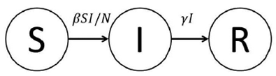
In a classic model SIR , individuals within the population N belong to one of three compartments: susceptible, infected, and removed, which are denoted by S, I, and R, respectively. These groups are defined as follows, the susceptibles: those susceptible to contract the disease, but who are not yet infected at a time t, the infected: those which are infected with the disease, and are able to spread it through contact with susceptibles. The final class are the removed: those that have been removed from the infected and cannot spread the infection (for instance, because they are immunized).
The following hypotheses are assumed: 1) it is considered a homogeneous
population without demographic dynamic, in which individuals have the same
characteristics; age, sexual gender, among others, 2) it is neglected a possible
seasonal period in which the dynamics of the epidemic vary, 3) it is excluded
the possibility that the removed individuals lose their immunity to the disease
so that they cannot belong to the susceptible group again, 4) it is ignored the
virus incubation time, which implies that when a subject is infected it becomes
infectious immediately, 5) it is considered that two individuals have the same
probability of interacting each other, 6) it is supposed that infected persons,
that are within the incubation period but do not exhibit any symptoms, are
unable to contaminate to other individuals, 7) the rate of the number of
infected per unit of time increases proportionally to the number of infected and
susceptible, namely
2.2.Governing equations
Under the conditions mentioned above, the model can be mathematically expressed by the following set of ordinary differential equations,
where N = S + I + R is the fixed total population. If everyone is initially
susceptible (S(0) = N), then a newly introduced infected individual can be
expected to infect other people at the rate βN during the expected infectious
period 1/γ. Thus, this first infected individual can be expected to infect
2.3.General master equation
The master equation governs the stochastic dynamics of Markov process. This equation is universal and has been applied in problems in biology and population dynamics which can be modeled as Markovian events. A process is considered Markovian if it is possible to make predictions and indeed know the full history of the process about the system, based solely on its present state, which implies that the past and future state of the system are independent. Therefore, a suitable description for Markovian systems is given by the master equation, that specifies how the probability P(ni, t) that the system is in the state ni at time t changes with time. Its general form is given by,
Equation (2) manifests explicitly that the temporal changes of the probability
are controlled by a balance equation that takes into account both transition
probabilities per unit time
2.4.One step master equation
In what follows, the description done so far on the master equation, will be limited only to the three population groups: susceptible, infected, and removed, as was discussed above are denoted by S, I, and R, respectively. We also will consider that an individual only has interaction with their nearest neighbour.
We suppose that the transition rule of the population members between the groups S, I, R is as follows: The susceptible individuals, initially healthy, may become infected with a rate ΒSI/N, whereas the infected individuals, have the disease and are able to transmit it to other individuals at a rate γI, the removed individuals are immune to the disease after recovery. For simplicity in this model, it is assumed that during the epidemic, the virus is transmitted only between close neighbours with the possibility that an infected individual may be removed. Figure 1 illustrates schematically the transition flows from one group to another.
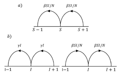
The elementary processes occurring into the system can be divided in two elementary groups; infection and recovery, which are defined as follows: An infection process implies that a susceptible individual enters in contact with an infected individual, generating therefore a newly infected individual. The recovery process signifies that an infected individual who is able to recover from the disease, cannot be susceptible again, because he has acquired immunity. In summary, the transition rates expressed in terms of the SIR model variables are defined by the following events,
which are represented schematically in Fig.
2 together with their respective transition rates. We take just two
variables
Equation (4) is a master equation describing a one-step process, whose corresponding associated transition rates we shall assume by proposing the following expressions,
Here, T (S -1,I +1 | S,I) measures the probability rate for an infected
individual to become susceptible I, while the number of removed R is constant.
We take this quantity to be proportional to the temporal rate of change of S
provided by the Kermack McKendrick model, as given by the first equation of Eq.
(1), which is conceptually resembling. Similarly, T(S,I -1 | S,I) gives the
transition probability at which the number of infected individuals increase by
one while the susceptible ones is kept constant. Because the total number is
constant, this is related with the reduction of the recovery individuals R whose
temporal ratio is provided by the last equation of Eq. (1). We identify both
quantities as proportional to construct our master equation. For convenience,
the one-step operator 𝐸, is defined through its effect on an arbitrary function
f(m) as
and
From transition rates represented by expressions (7) and (8), Eq. (4) can be written in a compact form as
In order to solve Eq. (9), we use the method that has been proposed by 13. This method suppose that the probability distribution P behaves like a sharp Gaussian statistical distribution, where the random variables are rewritten as the superposition of a macroscopic deterministic variable and a mesoscopic random variable. According to this formulation, the following ansatz for the independent variables are suggested, namely,
where
Inserting expressions (10-13) into Eq.9, and multiplying the hand right side by NP, it becomes
Notice that the expression between square brackets up to second order in q2 can be approximated as
Thus, if we expand the other terms and group the resulting ones in powers of q we can obtain
where the terms of order q have been neglected. It is important to remark that
Eq. (16) is the Fokker-Planck’s equation (see 13). Moreover, it is useful to express the
probability distribution in terms of S and I, which in turn can be written as a
function of the continuous variables x and y, namely,
By comparing the right hand side of the Eq. (16) and that of the Eq. (17), it can be infered by equating the lowest power in q that
Notice that the system of Eqs. (18-19), has the same functional form that SIR
model described by Eq. (1), whose solutions
which can be expressed as a continuity balance equation for the probability ∏ given by
where the two dimensional probability current vector
We remark that Eq.(21) guaratees the conservation of probability.
To analyze the dynamics of the expected values of the ramdom variables x and y we multiply by x or by y Eq.(20) and integrate over the whole domain. It yields
where as usual the expected value is given by
Here u is a variable which can be a function of x and y. By adding Eqs. (23) and (24) we get the expression
which allows us to find a time invariant of the system. To find the dynamics of
the second momenta, we proceed similarly and integrate by parts the resulting
expressions by assuming that the density of probability ∏ and its partial
derivatives with respect to x and y vanish at
After adding the first and second expressions and substracting the third one we obtain following relation
It is convenient to stress that the model described by the set of Eqs.(23), (24),
(27), (28), and (29) is general and therefore, it can be applied to any epidemic
of viral transmission fulfilling the restriction of having a narrow statistical
distribution; it means that he solution P(S,I,t) of Eq. (9) obeys a Gaussian
distribution with averages Φ(t) and ψ(t), whose fluctuations bands
3.Application of this model to study a realistic case
Before applying our stochastic formulation, it is good to mention that although the behavior of the groups S and R can be predicted by using a deterministic model, in contrast with infected group, its quantification for the whole population is very difficult, and, in consequence, there is not enough field data. The infected group is considered as the variable with more impact and as such, it is therefore the most commonly used in epidemiological predictions. For these reasons, we focus our discussion mainly in infected cases I.
In what follows, we apply the mathematical model developed in Sec. 2.1 and summarized by Eqs.
(23)-(29) to analize the influenza AH1N1 spread in Mexico in 2009. We use real data
reported by Mexican Institute for Social Security (IMSS) in that year. In Table I it is presented the total number of
infected people, this information includes 35 geographical regions stipulated by the
. We use the following methodology: even though it is well known that one
epidemiological year encompasses a whole period of 52 weeks, of which we only
consider those weeks in which there was a significant number of infected cases
N0. In regard to the proportion of the susceptible members
S(t), in the relation N(t) = S(t) + I(t) + R(t), it is taken those individuals who
finally became infected, which implies the initial condition I(t) = S(0) . In
addition, to estimate the order of magnitude of the parameters β and γ we apply the
Levenberg-Marquardt algorithm, whereas the value
Hence, the total number infected during the outbreak is
this implicit relation is used to calculate the number of susceptible people, by
using the Generalized Reduced Gradient (GRG) nonlinear algorithm. Also, for the
other expected variables we assume the following initial conditions:
4.Results and discussion
In Table I, we present the corresponding
values of the typical parameters β, γ, and
Table I Total number of cases and parameters estimated by geographical region 14.
| Geographical region | N | Infected cases | β | γ | R0 |
| Aguascalientes | 20,910 | 825 | 6.69 | 6.04 | 1.11 |
| Baja California | 43,918 | 1,050 | 9.98 | 9.64 | 1.03 |
| Baja California Sur | 11,289 | 565 | 5.82 | 5.13 | 1.13 |
| Campeche | 4,703 | 151 | 7.14 | 6.62 | 1.08 |
| Coahuila | 26,988 | 516 | 7.78 | 7.32 | 1.06 |
| Colima | 20,346 | 924 | 5.19 | 4.77 | 1.09 |
| Chiapas | 22,694 | 1,311 | 8.29 | 7.77 | 1.07 |
| Chihuahua | 21,309 | 458 | 9.56 | 8.85 | 1.08 |
| Durango | 17,154 | 752 | 5.00 | 4.43 | 1.13 |
| Guanajuato | 30,909 | 557 | 8.43 | 7.98 | 1.06 |
| Guerrero | 15,536 | 484 | 11.16 | 10.25 | 1.09 |
| Hidalgo | 15,193 | 758 | 6.58 | 5.71 | 1.15 |
| Jalisco | 91,003 | 1,576 | 8.52 | 8.12 | 1.05 |
| Mexico Oriente | 66,957 | 1,677 | 10.67 | 10.17 | 1.05 |
| Mexico Poniente | 40,153 | 1,245 | 7.21 | 6.55 | 1.10 |
| Michoacan | 22,708 | 607 | 6.76 | 6.25 | 1.08 |
| Morelos | 6,482 | 187 | 6.59 | 6.04 | 1.09 |
| Nayarit | 15,605 | 569 | 4.74 | 4.38 | 1.08 |
| Nuevo Leon | 69,512 | 1,571 | 10.49 | 10.01 | 1.05 |
| Oaxaca | 30,087 | 1,484 | 6.84 | 6.52 | 1.05 |
| Puebla | 24,470 | 685 | 8.54 | 7.79 | 1.10 |
| Queretaro | 30,237 | 834 | 8.91 | 8.59 | 1.04 |
| Quintana Roo | 6,365 | 203 | 17.25 | 15.43 | 1.12 |
| San Luis Potosi | 43,847 | 1,989 | 5.87 | 5.31 | 1.11 |
| Sinaloa | 17,395 | 441 | 7.82 | 7.14 | 1.09 |
| Sonora | 21,681 | 777 | 9.76 | 8.55 | 1.14 |
| Tabasco | 13,616 | 1,020 | 10.75 | 8.74 | 1.23 |
| Tamaulipas | 43,708 | 1,672 | 11.12 | 9.94 | 1.12 |
| Tlaxcala | 9,151 | 491 | 5.97 | 5.17 | 1.16 |
| Veracruz Norte | 29,404 | 749 | 10.54 | 9.82 | 1.07 |
| Veracruz Sur | 32,401 | 870 | 11.39 | 10.62 | 1.07 |
| Yucatan | 26,875 | 1,187 | 8.12 | 7.49 | 1.09 |
| Zacatecas | 9,915 | 385 | 8.85 | 7.94 | 1.11 |
| D.F. Norte | 60,936 | 2,063 | 11.18 | 10.68 | 1.05 |
| D.F. Sur | 52,399 | 1,253 | 8.09 | 7.47 | 1.08 |
| Whole country | 1,441,331 | 31,887 | 13.09 | 12.77 | 1.02 |
Figures 3-8 exhibit all the events that we have analyzed. The corresponding comparison between real infected cases I and its respective theoretical average E[I] has been presented for each geographical region. In the same Figs. 3-8, also is illustrated the corresponding associated curves with the extinction probability of the epidemic as a function of the time.
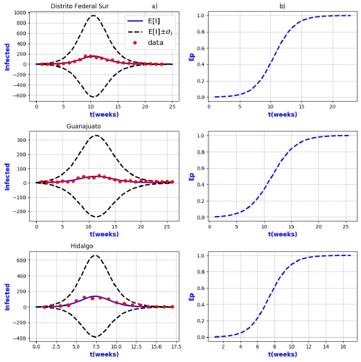
Figure 3 a) Probability distribution theoretical and observed. b) Ep=Extinction probability. Here ψ = E[I] is the expected value of the theoretical distribution and σ I is the standard deviation around the expected value.
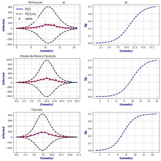
Figure 4 a) Probability distribution theoretical and observed. b) Ep=Extinction probability. Here ψ = E[I] is the expected value of the theoretical distribution and σ I is the standard deviation around the expected value.
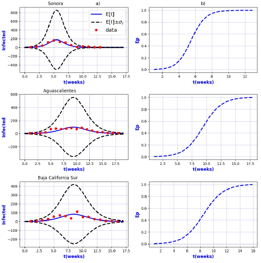
Figure 5 a) Probability distribution theoretical and observed. b) Ep=Extinction probability. Here ψ = E[I] is the expected value of the theoretical distribution and σ I is the standard deviation around the expected value.
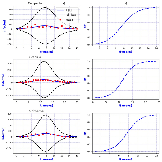
Figure 6 a) Probability distribution theoretical and observed. b) Ep=Extinction probability. Here ψ = E[I] is the expected value of the theoretical distribution and σ I is the standard deviation around the expected value.
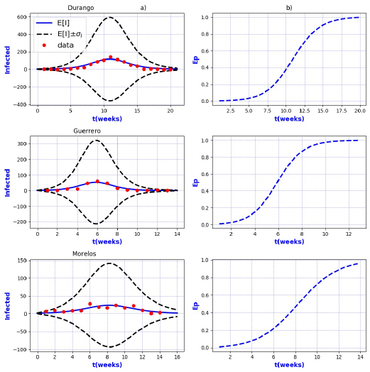
Figure 7 a) Probability distribution theoretical and observed. b) Ep=Extinction probability. Here ψ = E[I] is the expected value of the theoretical distribution and σ I is the standard deviation around the expected value.
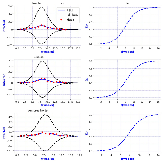
Figure 8 a) Probability distribution theoretical and observed. b) Ep=Extinction probability. Here ψ = E[I] is the expected value of the theoretical distribution and σ I is the standard deviation around the expected value.
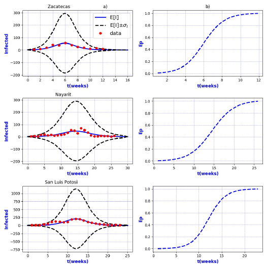
Figure 9 a) Probability distribution theoretical and observed. b) Ep=Extinction probability. Here ψ = E[I] is the expected value of the theoretical distribution and σ I is the standard deviation around the expected value.
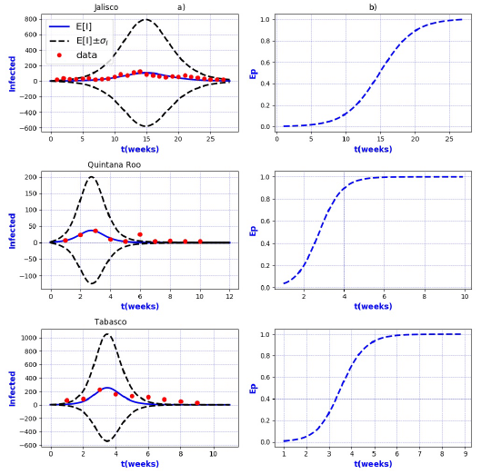
Figure 10 a) Probability distribution theoretical and observed. b) Ep=Extinction probability. Here ψ = E[I] is the expected value of the theoretical distribution and σ I is the standard deviation around the expected value.
The results show that the best fit correspond to geographical regions Distrito
Federal Sur, Guanajuato, Hidalgo, Michoacan, Estado de Mexico Poniente, Tlaxcala and
Sonora, because real data are accumulated around the expectation value E[I].
Moreover, the geographical regions Aguascalientes, Baja California Sur, Campeche,
Coahuila, Chihuahua, Durango, Guerrero, Morelos, Puebla, Sinaloa, Veracruz Norte,
Zacatecas, Nayarit, and San Luis Potosi, also exhibit a good fit with real data more
scattered around its theoretical average. However all of them are still within the
calculated probabilistic bands given by
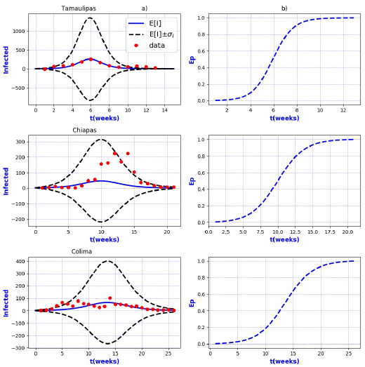
Figure 11 a) Probability distribution theoretical and observed. b) Ep=Extinction probability. Here ψ = E[I] is the expected value of the theoretical distribution and σ I is the standard deviation around the expected value.
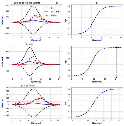
Figure 12 a) Probability distribution theoretical and observed. b) Ep=Extinction probability. Here ψ = E[I] is the expected value of the theoretical distribution and σ I is the standard deviation around the expected value.
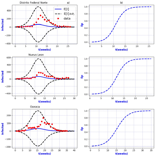
Figure 13 a) Probability distribution theoretical and observed. b) Ep=Extinction probability. Here ψ = E[I] is the expected value of the theoretical distribution and σ I is the standard deviation around the expected value.
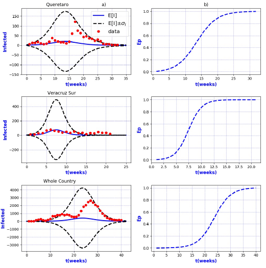
Figure 14 a) Probability distribution theoretical and observed. b) Ep=Extinction probability. Here ψ = E[I] is the expected value of the theoretical distribution and σ I is the standard deviation around the expected value
In contrast, the results show that the largest spread of real cases around the
theoretical average E[I] correspond to geographical regions Chiapas, Colima, Estado
de Mexico Oriente, Yucatan, Baja California, Distrito Federal Norte, Nuevo Leon,
Oaxaca, Queretaro, and Veracruz Sur as well as for the whole country. It can seen
that in some of these regions and in the whole country, a considerable number of
real cases are outside of the theoretical standard deviation bands
On the other hand, it is also important to point out that in the geographical regions Puebla, Sinaloa, Colima, Jalisco, Estado de Mexico Oriente, Nayarit, San Luis Potosi, Yucatan, Distrito Federal Norte, Nuevo Leon, Oaxaca, Queretaro, and Veracruz Sur an oscillatory trend is observed particularly notorious at the level of the entire country. The origin of these discrepancies probably, is owing to two main reasons: 1) the simplicity of the model that we have utilized and / or 2) inaccuracies in the acquisition of field data. A possible solution in order to have a better fit, could be the implementation of a more realistic model that takes into account infected death, vaccination, births, population migration, incubation period of the virus, among other factors which we have neglected. Moreover, the oscillatory behavior observed, characteristic in large populations, suggests the necessity of introducing seasonal forcing into the model. In parallel, suitably trained staff would represent a direct improvement on the quality and reliability of the data.
In regard to extinction probability as a function of time, we have identified the week for which there is a 90% of extinction probability of the epidemic -a threshold that has been chosen arbitrarily and could easily be changed-. Under this criteria, the average extinction time for each geographical region as well as for whole country was around 13 and 30 weeks respectively. Moreover, geographical regions in which it is observed a longer period of extinction corresponding to 90% are, Colima, Nayarit, and Queretaro with 19 weeks, Jalisco and Baja California with 20 weeks and Oaxaca with 21 weeks. Complementary, shorter periods were found for geographical regions Quintana Roo and Tabasco with 4 weeks.
As already mentioned, these estimates values could be improved with the implementation of a more realistic model and a more reliable registration of infected cases. However, a lot of the neglected processes and unrevealed variables can be incorporated to some extent, within the standard deviation band that we have computed. This is indeed the power of our stochastic approach because even though there exist various additional variables, not considered here, which modify our epidemic evolution, we can embody all of them within the statistical distribution of the parameters of a quite simple dynamic model which describes the dominant behavior of the phenomenon.
5.Concluding remarks
We have established a stochastic model based on a simple compartmental SIR formalism. Using this approach we have studied the propagation of the AH1N1 influenza that took place in Mexico in 2009. We have restricted this study to
fected cases reported by Mexican Institute for Social Security (IMSS) in that year.
Our main conclusions are the following: the order of magnitude estimated for the
basic reproductive number of infection
As future work, it will be interesting to formally extend the present study by including the main health agencies that have a presence throughout the country, such as the Mexican Secretariat of Health (SSA), Institute for Social Security and Services for State Workers (ISSSTE) and Navy Secretariat (SEMAR). The data set coming from these institutions would complement the information provided by the Mexican Institute for Social Security (IMSS) for a nationwide study. We can even consider other kind of epidemics, as well as an extension to our model by means of incorporating important variables such as: vaccination, demographic dynamics (emigration, immigration, births, and deaths), information on passive immunity, age and sex of the population, quarantine period, incubation period of the infectious agent, loss of immunity, forcing seasonal, among other factors. It would also be interesting to consider an interaction between individuals beyond their immediate neighbors, that is, second and third neighbors. Nevertheless, we should be aware of including only a few additional important variables in order to keep a very simple and easy-to-use description.

