


 nueva página del texto (beta)
 Inglés (pdf)
 Artículo en XML
 Referencias del artículo
 Enviar artículo por email
 Citado por SciELO
  Similares en
SciELO
Similares en
SciELO 
 Permalink
1. Introduction
The first chaotic system was introduced by Edward Lorenz [1]. From this, the interest in developing new similar systems emerged, and it has been applied in several applications such as securing communications [2], synchronization of systems [3], power systems [4], among others. In dynamical systems, equilibrium is an important characteristic, since the motion of trajectories depend on the local behavior around the neighborhood of the fixed point. Most of the chaotic systems reported in the literature have a determined number of equilibria, and these have been widely studied. For instance, the Lorenz [1], Chen [5], Lü [6] and Chua [7] systems have three equilibrium points, and the Rössler system [8] has only two equilibrium points. Likewise, Sprott [9] has proposed a set of chaotic systems where some of them have only one or two equilibrium points. Moreover, some chaotic systems have an equilibrium point in each basin of attraction which is generated by a piecewise linear function (PWL) [10-12]. The PWL function allows to obtain a set of linear systems, each one having a hyperbolic equilibrium point. These systems can generate three or more scrolls in an attractor; thus, they are known as multi scroll attractors.
Similar systems have been studied with two or more positive Lyapunov exponents. According to [13], these dynamical systems are called hyperchaotic.
In recent years, some systems that generate chaotic attractors which their basin of attraction does not intersect with its neighborhoods of the equilibrium points have been found, these are known as hidden attractors. Hidden attractors are difficult to find because both basins of attraction and the dimension of the attractor could be very small. According to [14], the systems with hidden attractors are classified as a hidden attractor without equilibrium, a hidden attractor with an infinite number of equilibria, and a hidden attractor with one stable equilibrium. For these systems, it is not possible to apply the Shilnikov theorem [15, 16] to demonstrate the existence of chaos, because they do not have homoclinic and heteroclinic orbits.
From Sprott’s A-system [9], chaotic systems without equilibrium such as Pham [17], C. Wang [18], Azar [19], Wei [20] and Jafari [21] systems have been developed. Also, hyperchaotic systems [22], multi scroll systems [23-25], and fractional-order systems [26, 27] without equilibrium have been studied.
On the other hand, some authors have developed chaotic systems that present an infinite number of equilibria. For instance, Jafari [28], Chumbiao [29] and Li [30] systems. Besides it has been found that some hyperchaotic systems [31] and fractal-order systems [32] has a line of equilibria.
Finally, the systems with only one stable equilibrium have been studied from the Sprott’s E-system. Some authors, such as Wang [33], Pham [34], among others, proposed similar systems through quadratic nonlinearities. Also, systems with two stable equilibria [35, 36] have been developed, and this opens the possibility to design multi scroll systems in the future.
Notice that the chaotic systems mentioned above present quadratic nonlinearities. However, there are a few systems in the literature that generate hidden attractors from switching linear systems [37,38]. In these researches, the main methodology is to find hidden degeneracies in piecewise smooth dynamical systems through the sliding mode methods, and they use of efficient analytical-numerical methods for the study of hidden attractors. The approach is based on the use of modern computers and the development of numerical methods. Chua’s system was used to find hidden attractors trough these approaches. Due to this motivation, this work presents a new methodology to develop a family of three-dimensional hidden attractors from the switching linear systems. The Rouché-Frobenius theorem is used as a tool to analyze the equilibrium of every switching system. Thus, these systems can generate a chaotic system without equilibrium, a chaotic system with an infinite number of equilibrium points, or a chaotic with a stable equilibrium.
This paper is organized as follows: In Sec. 2, the preliminary theory of linear systems is introduced, and its relationship with the equilibrium of the dynamical system. The switched systems without equilibrium, with an infinite number of equilibria, and with stable equilibrium are introduced in Secs. 3 to 5. Finally, a discussion of the proposed systems and the conclusions are given in Secs. 6 and 7, respectively.
2. Equilibrium description of a linear system
This section contains briefly the study of the equilibrium point of a linear system, and its main features are presented. Consider a three-dimensional linear dynamical system given by
where x = [x 1 ,x 2 ,x 3] T ∈ R3 is the state variable, B = [b 1 ,b 2 ,b 3] T ∈ R3 stands for a vector of real constants and A ∈ R3×3 is a linear operator given by
Assume the system (1) is dissipative; that means, the sum of its eigenvalues is negative, and it has stable (W S ) and unstable (W U ) manifolds. The behavior of the system is defined through the eigenvalues of A, which are obtained from the characteristic polynomial
where β = α 11+α 22+α 33, γ = α 11 α 22+α 11 α 33+α 22 α 33− α 12 α 21 − α 13 α 31 − α 23 α 32 and δ = det(A). The eigenvalues of the system are determined through the discriminant of the polynomial g(λ). By definition, the discriminant of a thirddegree polynomial is as follows
where the next cases are considered: (1) if ∆ > 0, the dynamical system (1) has three different eigenvalues; (2) if ∆ = 0, the dynamical system (1) has multiple eigenvalues; and (3) if ∆ < 0, the dynamical system (1) has a real eigenvalue and a pair of complex-conjugate eigenvalues.
The algebraic linear system solution (5), it is a starting point to analyze the equilibrium of the system, since both concepts are strongly related.
The Rouche-Frobenius theorem uses an augmented matrix (A|B), and provides the necessary conditions to establish the type of solution. The concept of equilibrium point and theorem are related as follows:
The linear system (5) has a unique solution, if and only if, the rank(A) = 3 and rank(A|B) = 3. In other words, a unique solution exists if A is not singular. Hence, the dynamical system (1) has a hyperbolic equilibrium point given by x * = −A −1 B, and the eigenvalues of matrix A have the nonzero real part. Therefore, the system (1) is called a hyperbolic linear system.
The linear system (5) has multiple solutions if the rank(A) = rank(A|B) < 3, that means, the matrix A is singular. Consequently, the dynamical system (1) has an infinite number of equilibrium points. Because of that the constant term δ = 0 and ∆ < 0 in Eq. (3), the system is nonhyperbolic, since at least one of its eigenvalues has the real part equal zero.
Finally, the linear system (5) does not have a solution if the rank(A) ≠ rank(A|B), consequently, det(A) = 0. Thus, the dynamical system (1) does not have equilibrium, and it is nonhyperbolic since at least one of its eigenvalues has the real part equal zero.
The first statement from the aforementioned theorem is the main characteristic of a self-excited attractor since its basin of attraction intersects with the neighborhood of the equilibrium point. On the other hand, the last two statements are related to hidden attractors. That means its basin of attraction does not intersect with the neighborhoods of equilibria. It is important to mention that the systems with a stable equilibrium fulfill the first statement of the Rouché-Frobenius theorem, however, they are considered as hidden attractors. The previous theorem is considered along with this paper since we pretend to generate a chaotic attractor through the switching of nonhyperbolic linear systems.
3. Switched chaotic system without equilibrium
This section introduces to a system without equilibrium from the switching of two nonhyperbolic linear systems. Each linear system A i x = B i belongs to domain D i ⊆ R3, where the matrix A must be singular.
Assume that the flow of the switching system is given by x(t) = φ(x 0) such that t ≥ 0. Moreover, assume that the system is dissipative and generates an attractor. As a case study, consider the next switching system
The domain of the system is D1 when x 1 ≥ 0 and D2 when x 1 < 0. The states vector x and the vectors B 1 and B 2 are defined in Eq. (1). Finally, the matrices A 1 and A 2 are given by
Both previous matrices have a column vector zero, thus, det(A 1) = det(A 2) = 0. This leads to the third statement of Rouché-Frobenius theorem, if and only if, the elements of´ B 1 and B 2 are nonzero. Then, this guarantees that the system (6) does not have equilibrium.
To obtain a chaotic behavior, firstly, the solution of the initial value problem must be of an oscillatory nature through of the eigenvalues. The characteristic polynomials associated with D1 and D2 are shown in the Eq. (8); meanwhile, their eigenvalues are given in the Eq. (9).
Note that these matrices have an eigenvalue equal to zero because g(λ) and g(µ) do not have independent terms. Thus, the solution set is of oscillatory nature if the last two eigenvalues are one pair of complex-conjugates, that is to say, (p + k)2 < 4(q 2 + kp) and (p − k)2 < 4(q 2 − kp), for D1 and D2, respectively. Therefore, according to Eq. (4) the discriminant is calculated as ∆ = β 2 γ 2 − 4γ 3 < 0.
Let p = 0.25 and q = 3 be the elements of matrices A 1 and A 2, and let b 1 = b 2 = 0 and b 3 = 0.05 be elements of vectors B 1 and B 2. Taking into account the above inequalities, the parameter k is defined through a systematic search assisted by software based on the methods proposed in Ref. [39]. This search consists in to find both the value of k as the initial conditions, such that the Lyapunov exponents or the bifurcation diagrams show the presence of chaos in the system.
In this way, the system (6) has chaotic behavior when the parameter k = 2.3 and the initial conditions are (x 10 ,x 20 ,x 30) = (0.05,0.05,0.05). The properties of the characteristic polynomials of the domains D1 and D2 were verified. In the domain D1, the discriminant is ∆ = −2915.21 and the eigenvalues associated are λ 1 = 0 and λ 2,3 = −1.275 ± 2.8195i. Meanwhile, in the domain D2, the discriminant is ∆ = −2093.75 and the eigenvalues are µ 1 = 0 and µ 2,3 = 1.025 ± 2.7156i.
The Lyapunov exponents are denoted by λ L1 = 0.1086, λ L2 = 0 and λ L3 = −0.3509, and the Kaplan-Yorke dimension is D KY = 2.3065, which indicate that there exist a strange attractor. The sum of Lyapunov exponents λ L1 + λ L2 + λ L3 = −0.2423 indicates the system is dissipative. However, the dissipation of each domain is calculated by the variation of a small element of volume V (t) as
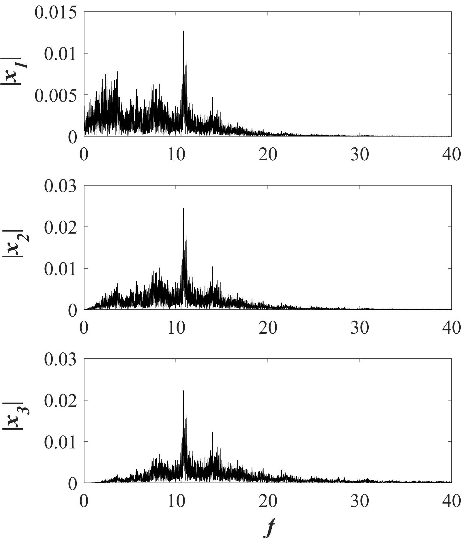
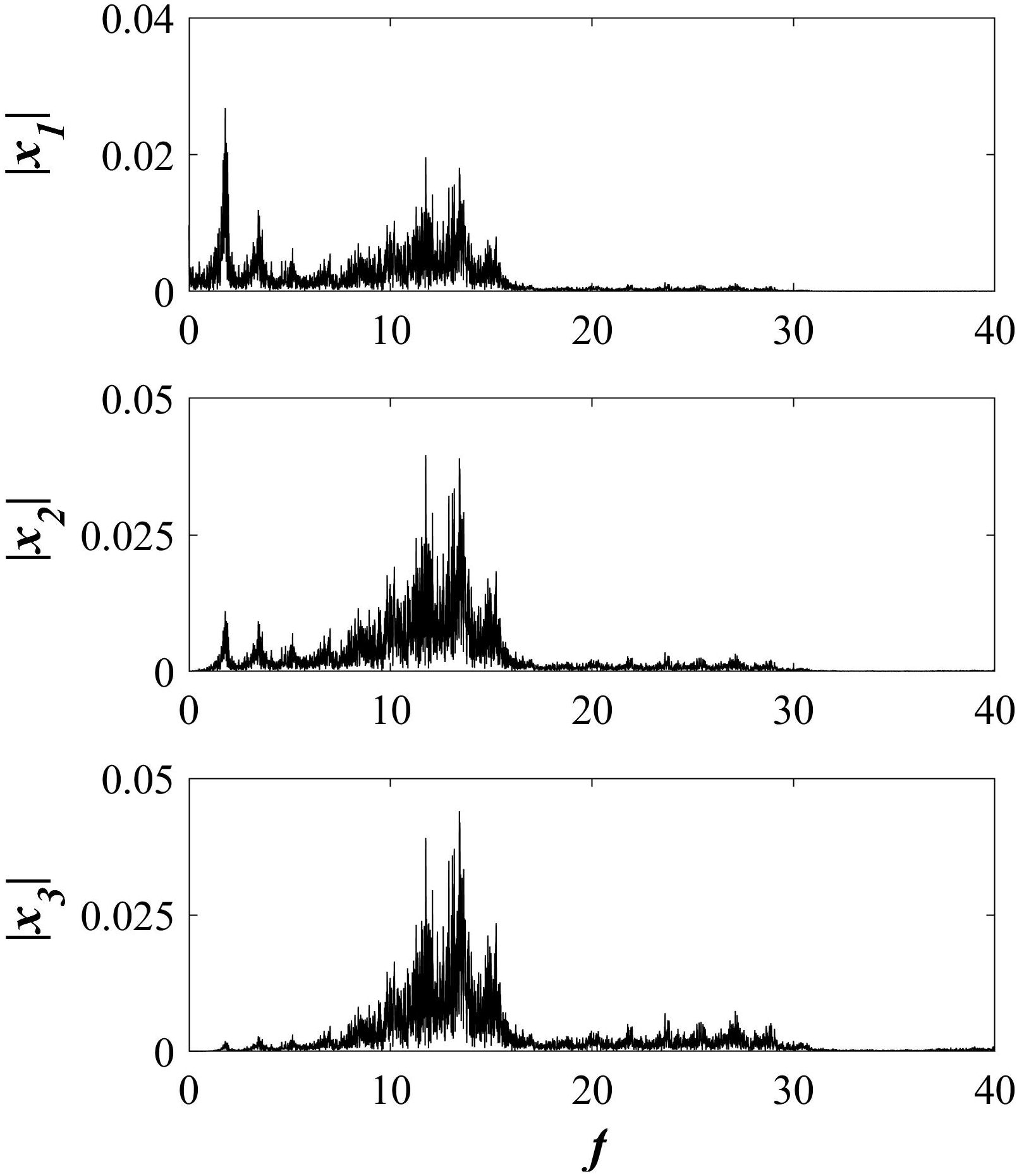
In Fig. 1, it is can observe the time series of states x 1, x 2, and x 3. Also, the hidden attractor generated from the switching system is shown. The frequency spectra of the time series confirm that they are of a chaotic nature in Fig. 2.
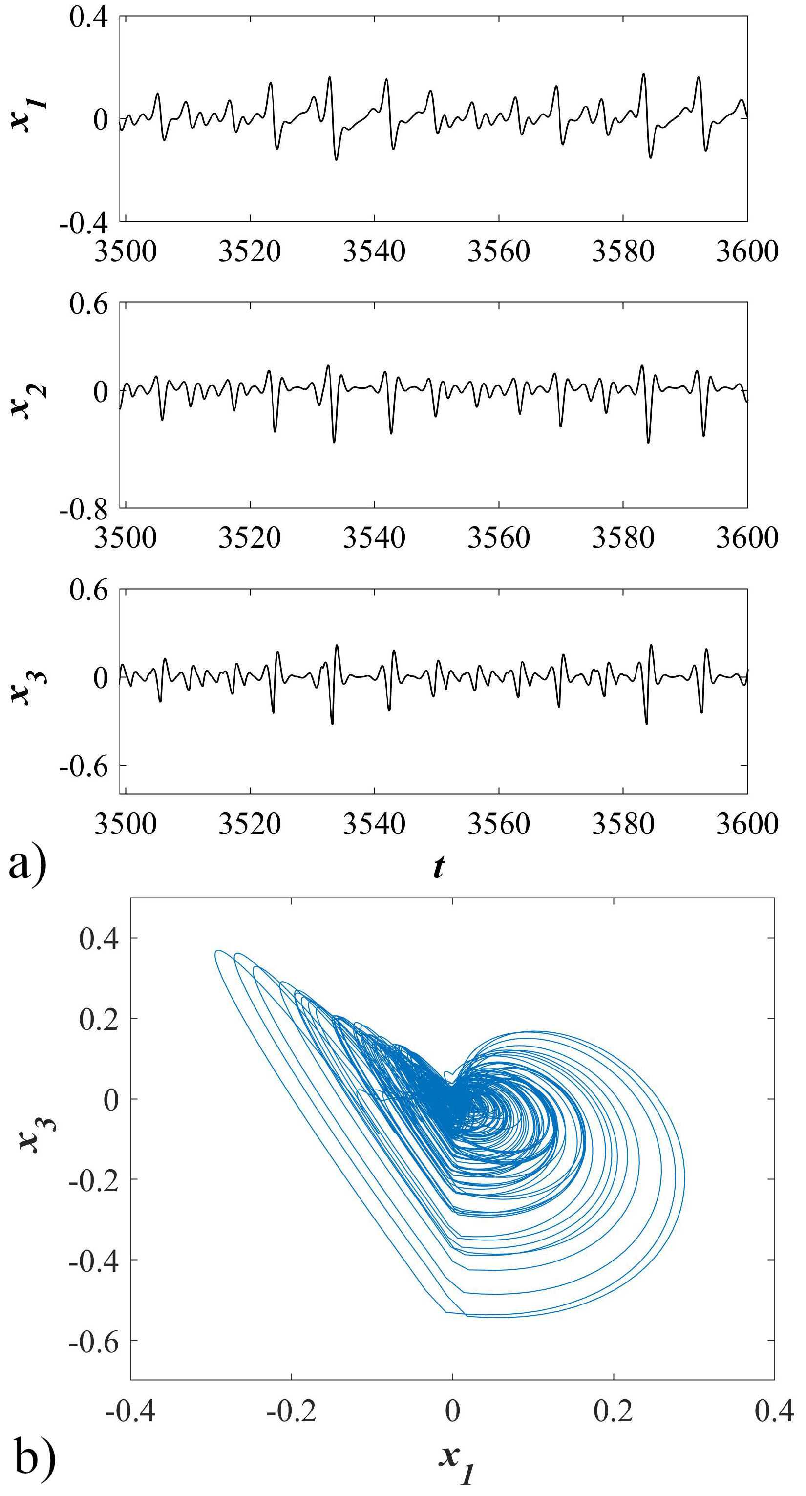
FIGURE 1 a) Time series of states of the switching system without equilibrium. b) Phase portrait of the chaotic attractor in the switching system without equilibrium on x 1 − x 3-plane.
4. A switched chaotic system with an infinite number of equilibrium points
This section presents the switching of a linear system with an infinite number of equilibria and a linear system without equilibrium. Hence, the equilibrium of the switched dynamical system is an infinite number of equilibrium points. Consider the next system
where x = (x 1 ,x 2 ,x 3) is the states vector, and the matrices are denoted by
Both matrices have det(A 3) = det(A 4) = 0. The domain of system (11) is represented by D3 when x 1 ≥ 0 and D4 when x 1 < 0. The domain D3 has an infinite number of equilibrium points, if and only if, B 3 = (0,0,0) T . This leads to the second statement of Rouché-Frobenius. The equilibrium´ of D3 has been obtained when the following algebraic equations are solved:
Thus, the equilibrium is defined by
According to equation (3), the characteristic polynomials of the matrices in (12) are as follows
Then the discriminant of g(λ) and g(µ) is ∆ = β 2 γ 2 − 4γ 3. Thus, their corresponding eigenvalues are defined by
Like in the previous section, domains should be governed by eigenvalues such as unstable focus or stable focus. This provides an oscillatory solution to the initial value problem. This implies the next inequalities from Eq. (15) (k 3 − p)2 < 4(k 1 q − k 3 p) and (k 3 − p)2 < 4(k 2 q − k 3 p) in D3 and D4, respectively.
Assume that the parameters of the system (11) are p = 0.25, q = 3, b 3 = 0.2, and k 3 = 1.75. According to the inequalities aforementioned, we have an unstable focus and a stable focus when the parameters k 1 > (1/3) and k 2 > (1/3), respectively. In the same way, the initial conditions and the parameters k 1 and k 2 are found through the systematic search by software. Chaotic behavior was found when k 1 = 1.9 and k 2 = 4.1 with initial conditions (x 10 ,x 20 ,x 30) = (0.05,0.05,0.05). The eigenvalues of domain D3 are λ 1 = 0 and λ 2,3 = 0.75 ± 2.1679i with ∆ = −520.645. On the domain D4 their eigenvalues are µ 1 = 0 and µ 2,3 = −0.75 ± 3.3615i with ∆ = −6360.49.
The Lyapunov exponents of the switched system with an infinite number of equilibrium points are λ L1 = 0.04298, λ L2 = 0 and λ L3 = −0.1129, and the Kaplan -Yorke dimension is D KY = 2.38070. This confirms the presence of chaos and the existence of a strange attractor. This system is dissipative since the sum of the Lyapunov exponents is negative, we have λ L1 + λ L2 + λ L3 = −0.0631. Meanwhile, the divergence and convergence of the flow of each domain are obtained in Eq. (16). It is clear that domain D4 is dissipative, but D3 is not.
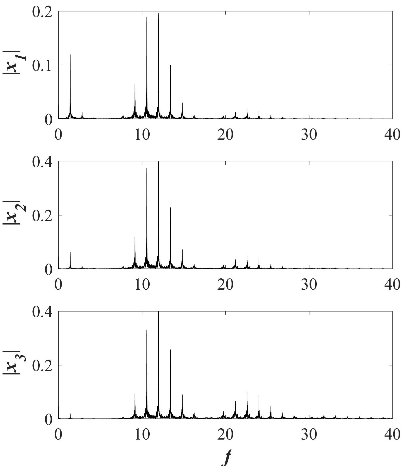
Figure 3 shows a section of the times series of states x 1, x 2 and x 3, moreover, the phase portrait of the hidden attractor on x 1 − x 3 plane is present. The frequency spectra for each time series are illustrated in Fig. 4.
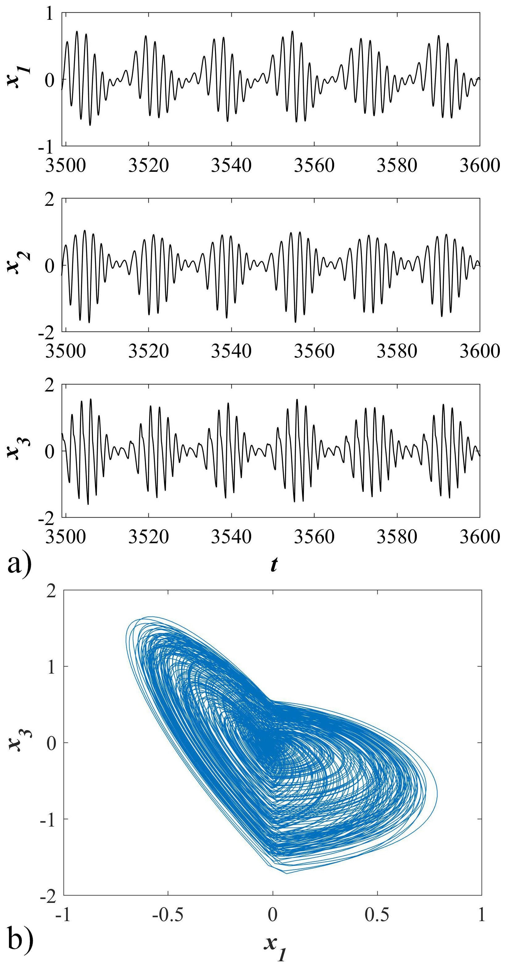
FIGURE 3 a) Time series of states of the switching system with an infinite number of equilibrium points. b) Phase portrait of the chaotic attractor in switching system with an infinite number of equilibrium points on x 1 − x 3-plane.
5. Switched chaotic system with only one stable equilibrium point
This system is developed by the switching of a linear system without equilibrium and a linear system with one stable equilibrium. To analyze this case, a switching system is proposed as follows
where the matrices A 5 and A 6 are given by
and the values of the parameters p and q are the same as the previous sections.
The linear system A 5 x+B 5 does not have an equilibrium, if and only if, B 5 = (0,0,b 3) T , with b 3 ≠ 0. This system was studied in detail in Sec. 3 as well as their eigenvalues. On the other hand, the system A 6 x+B 6 with B 6 = (0,0,0) T has one equilibrium point when the next algebraic system is solved,
Thus, this linear system has one equilibrium point in E(0,0,0). This equilibrium must be stable, which means, all the eigenvalues associated with the matrix A 6 must have a negative real part. Therefore the system (17) has one equilibrium point.
Now, the analysis of the matrix A 6 is carried out from the characteristic polynomial
This polynomial has an independent term, that means, the determinant of the matrix A 6 is nonzero. Thus, Cardano’s method is used to solve the polynomial. Consider the next cubic equation
where parameters are α = (k 1 + p), b = (k 1 p + q 2 + k 2) and c = k 2(p + q). Now, we perform a change of variable as follows:
and substituting in Eq. (21) the quadratic term is removed. Hence, the reduced cubic equation is obtained
where
The cubic Eq. (23) has three roots, and they are calculated as follows:
where the values of parameters P y Q are defined as
Finally, the roots of Eq. (21) are calculated from the solutions of Eq. (23). Consequently, we have
Notice that the parameter σ is equivalent to the discriminant in Eq. (4). Then, the matrix A 6 has a real eigenvalue λ 1 and a pair of complex-conjugate eigenvalues λ 2,3 if σ > 0.
Taking into account the mathematical expressions above, the values of the parameters k 1 and k 2 are found, by a systematic search, such that all eigenvalues have the negative real part. The system (17) is chaotic and has an equilibrium stable when k 1 = 2 and k 2 = 2.6, with the initial conditions (x 10 ,x 20 ,x 30) = (0.05,0.05,0.05). Analyzing the local behavior in x 1 ≥ 0, the eigenvalues of g 5(µ) (it was studied in detail in Sec. 3) are µ 1 = 0 and µ 2,3 = 0.875 ± 2.7811i with ∆ = −2235.23. Hence, in x 1 < 0, the eigenvalues of g 6(λ) are λ 1 = −0.7710 and λ 2,3 = −0.7395±3.2270i with ∆ = −4516.99.
This system is chaotic because the Lyapunov exponents are λ L1 = 0.3562, λ L2 = 0 and λ L3 = −0.5560, and the existence of the strange attractor is confirmed by the Kaplan-Yorke dimension, D KY = 2.6548. Besides the system dissipation is verified by the sum of the system of the Lyapunov exponents is negative and is λ L1 + λ L2 + λ L3 = −0.1998. Thus, the divergence of the flow of each domain is
The time series and chaotic attractor are presented in Fig. 5. As can be seen in Fig. 6, frequency spectra indicate the chaoticity of the system.
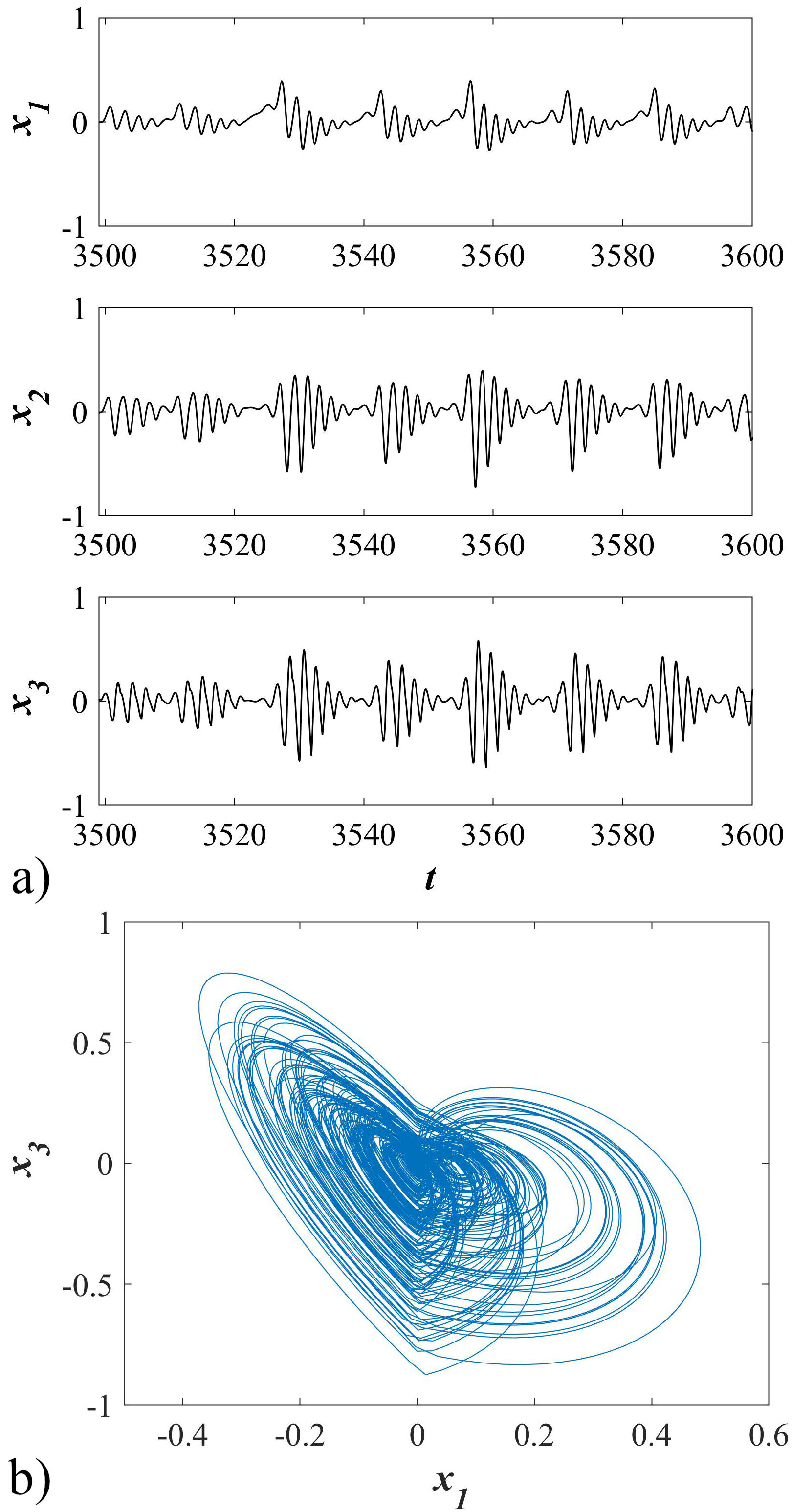
FIGURE 5 a) Time series of states of the switching system with only one stable equilibrium point. b) Phase portrait of the chaotic attractor in a switching system with only one stable equilibrium point on x 1 − x 3-plane.
6. Discussion
The dynamic of the previous systems was analyzed through the parameter variation found by the systematic search. For the switching system without equilibrium, the parameter k was varied in the interval from 2 to 5. Figure 7 shows the system dynamics through the Lyapunov exponents. As can be observed, the chaoticity exists in the system for some values into the intervals from and 2.1 to 2.5 and from 2.9 to 3.2.
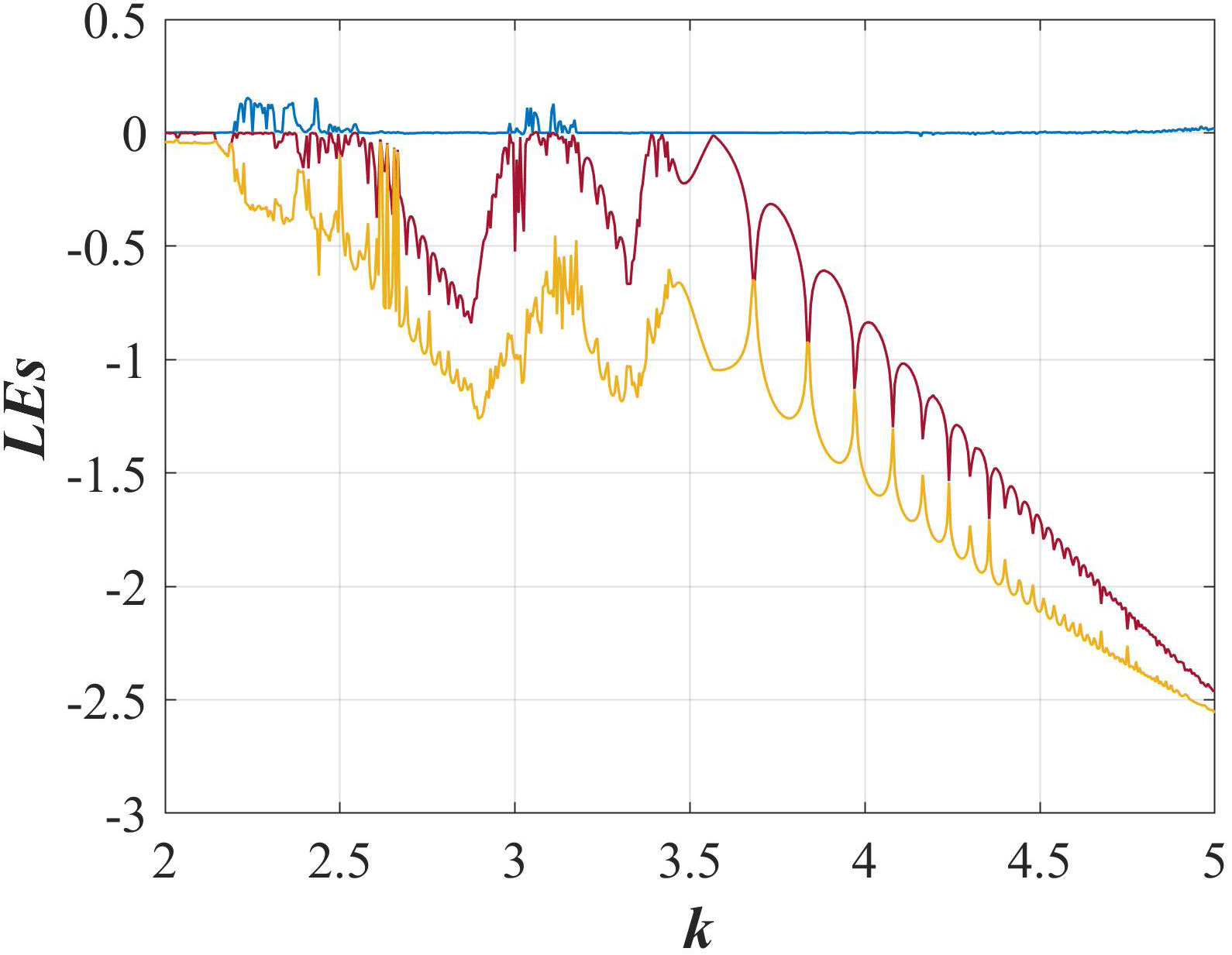
FIGURE 7 Dynamic of the Lyapunov exponents of the switching system without equilibrium when parameter k is varied from 2 to 5.
For the switching system with an infinite number of equilibrium points, its dynamic has been plotted in a Lyapunov exponents diagram (Fig. 8) concerning parameter k 1 when is varied from 1.5 to 5. It can be observed a small region of chaos from 1.6 to 2.2, though limit cycles exist in the interval from 2.2 to 5. However, note that the system power spectrum presented in Sec. 4 (Fig. 4) shows strong amplitude peaks. Also, the Lyapunov exponents are very small, and its almost impossible to distinguish from zero, this indicates the strong probability that the system with an infinite of equilibrium points may be a quasi-periodic. In this way, not only can beautiful chaotic systems can be obtained by mixing linear systems, but even quasi-periodic dynamics can be obtained as well.
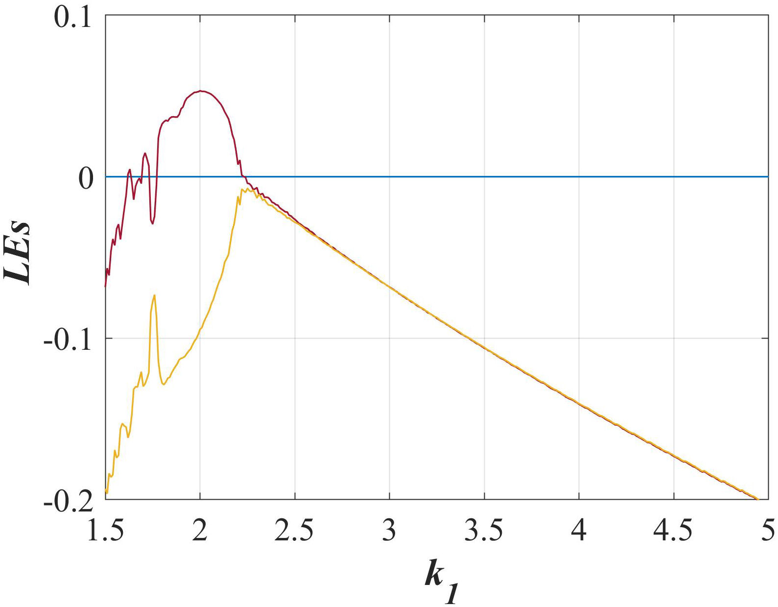
FIGURE 8 Dynamic of the Lyapunov exponents of the switching system with an infinite number of equilibria when k 2 = 4.1 and k 1 is varied from 1.5 to 5.
Similarly, a Lyapunov exponents diagram has been plotted in Fig. 9 to the switching system with only one stable equilibrium, where the parameter k 2 was varied from 0 to 4.5. It can be appreciated that the region to k 2 > 2.5, some values indicate chaos in the system.
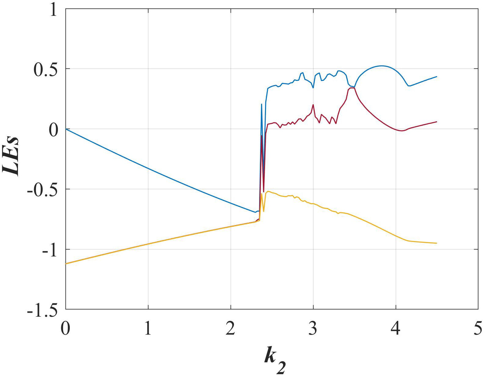
FIGURE 9 Dynamic of the Lyapunov exponents of the switching system with only one stable equilibrium when k 1 = 2 and k 2 is varied from 0 to 4.5.
It is hard work to find chaotic behavior in a switching system, and generate hidden
attractor since they are developed from the combination of linear systems
no-solution, multiple solutions, or a unique solution when
Despite this, we have found that the dynamics of these systems are bounded and converges towards the attractor for a wide range of initial conditions and different system parameters. Table I summarized some cases of the switching systems above (with different values of their parameters), where chaos is present. The system without equilibrium is stood for SW NE , the system with many equilibria as SW LE and the system with one stable equilibrium as SW SE .
TABLE I Three cases derived from the switching systems presented previously, for the initial conditions (x10, x20, x30) = (0.05,0.05,0.05).
| Case | Parameters | Equilibrium | Eigenvalues | LEs | DKY |
| SWNE | k = 3.11 | None |
µ1 = 0 µ2,3 = −1.68±2.6372i λ1 = 0 λ2,3 = 1.43±2.4854i |
λL1 = 0.1214 λL2 = 0 λL3 = −0.7168 |
2.1682 |
| SWLE |
k1 = 2 k2 = 4.1 k3 = 1.75 |
E(x*,0,0) |
µ1 = 0 µ2,3 = 0.75±2.2360i λ1 = 0 λ2,3 = −0.75±3.3615i |
λL1 = 0.0527 λL2 = 0 λL3 = −0.0939 |
2.5611 |
| SWSE |
k1 = 2 k2 = 4 |
E(0,0,0) |
µ1 = 0 µ2,3 = 0.875±2.7810i λ1 = −0.9371 λ2,3 = −0.4064±3.4019i |
λL1 = 0.4849 λL2 = 0 λL3 = −0.8892 |
2.5374 |
The above dynamics systems were numerically solved by the fifth-order Rungé-Kutta method. The simulations were generated in a time interval from 0 to 5000 with an integration step dt=0.001. On the other hand, the systematic search mentioned in each section above is based on the methods proposed in the reference [39]. This search consists in to find both the values of some parameters as the initial conditions, such that the Lyapunov exponents show the presence of chaos in the system. The Lyapunov exponents were calculated using the algorithm of Wolf [40], and they were verified using the algorithm from the reference [41].
7. Conclusions
A family of switching systems that generates hidden attractors is proposed in this paper. The presence of stable equilibrium, an infinite number of equilibria, and no-equilibrium is in this family. The development of these switching systems is based on the linear systems theory. It is important to mention that most of the hidden attractors reported in the literature are constructed by systems with quadratic nonlinearities. However, a few hidden attractors constructed through the switching of linear systems have been found in the literature. It would be interesting to implement these systems on chaos-based applications.

