


 nueva página del texto (beta)
 Inglés (pdf)
 Artículo en XML
 Referencias del artículo
 Enviar artículo por email
 Citado por SciELO
  Similares en
SciELO
Similares en
SciELO 
 Permalink
1. Introduction
The liquid-vapor equilibrium of substances in engineering applications is modeled mainly with cubic equations of state (CEoS). This approximation is practical and useful when the substances are fluids, but cubic equations cannot predict the solid phase [1]. In this case, solid phase and its coexistence states can be addressed using a pseudo-mixture instead of the substance per se, i.e. the substance is considered as a “mixture” [2-4] with two or more components of the same substance. In this approximation, the main component is constituted by single molecules of the substance, while other components are constituted by molecular clusters (solid phase). Such pseudo-component differs from other only by the size of molecular cluster. Thus, the liquid and the vapor phases are described by the CEoS of the substance, while the solid phase (constituted by different sets of molecular clusters) is described with its corresponding CEoS at the “mixture”.
Another approximation is by using a modified CEoS. The new equation of state is necessarily a Non-Cubic Equation of State (Non-CEoS). There are few analytical Non-CEoS in the literature [4-8], and all of them were designed to do possible a second loop to capture the solid-liquid coexistence (similar to the loop for the liquid-vapor coexistence in a conventional CEoS). The first example of a Non-CEoS corresponds to Wenzel’s equation [5], and its subsequent modification [9], that captures some solid-liquid coexistence states, but it was not designed to avoid a solid-liquid critical point. At least in the literature, there is not evidence about the occurrence of such solid-liquid critical point.
In the second example, Yokozeki’s equation introduces a factor with an un-physical discontinuity in the repulsion term (see ref [10]). This discontinuity was introduced to avoid a solid-liquid critical point in an effective way [6, 7], but is unnecessary and do not have a plausible physical interpretation [10]. The third and final example was reported by Guevara and Romero [8] and its structure will be given in equation (1a) in the following section. In this case, the most general CEoS is modified with an additional attractive term [11], and the procedure to define this term implies that solid-liquid critical point does not exist at all.
In this work, the equation developed by Guevara and Romero [8] was applied to several substances to obtain the parameters that define this equation for each substance, and some phase diagrams are calculated to compare the prediction of coexistence states with experimental data. The procedure to obtain an expression of the Non-CEoS for a particular substance is described in Sec. 2; while the database of substances and its associated parameters are reported in Sec. 3, along with some graphical examples of three of the substances reported. Conclusions are in Sec. 4.
2. Defining Non-CEoS
The Non-CEoS reported in [8] is showed in Eq. (1a):
In this case, the pressure P of the fluid is a function of the molar volume v, and the temperature T, while R is the gas constant (= 83.14472 cm3 bar/Kelvinmol). The Non-CEoS is composed by a cubic equation of state P 0 plus an attractive term that is related to very short-range interactions between molecules of the substance. Thus, the attractive term affects the behavior of cubic equation only at a neighborhood of the exclusion volume b. In other words, vapor phase predicted by cubic equation practically does not change, because the short attractive term is negligible. However, solid phase appears due to this attractive term and is additional to the liquid and vapor phases predicted by P 0.
Cubic equation of state P 0 (Eq. 1b) take account of the mean size of molecules through the parameter b. The effect of mean-range interactions between molecules is considered through the attractive term, and is implicitly included in the function a(T) through the second virial coefficient B(T). The relation between α(T) and B(T) comes from the virial expansion of the equation of state, as shown in Eqs. (1c) and (1d), and the expression of B(t) is the exact result derived from square-well potential (see Eq. (4), in Sec. 3). Square-well potential u(r) captures the main features of a mean-range attraction between molecules and describes the liquid-vapor coexistence.
Finally, in order to define the analytical expression of the Non-CEoS for a particular substance is necessary to obtain the set of parameters {b,c,d,e,f,λ,ε}. These parameters are determined using the following experimental data of the substance: critical pressure P c , critical molar volume v c , and critical temperature T c , the acentric factor ω, temperature T b at the boiling point, and temperature T t at the triple point. The exponent ν is also a parameter that can be adjusted according to the substance to be studied. For this work, an exponent of ν = 12 was found adequate to represent the complete phase transitions curves of the reported substances.
3. Procedure to construct the equation of state
The first step in order to define the Non-CEoS is finding the parameters (b,c,d) that appear in Eqs. (1a)-(1d), using the liquid-vapor critical point defined by the coordinates (P c ,v c ,T c ). The Non-CEoS needs to fulfills the following conditions:
To solve the previous system of equations is possible in the special case of a null attractive term in Eq. (1a), i.e. f = 0, that reduces (1a) to a cubic equation of state. In this case, parameters b, c, and d are determined from Eqs. (2a)(2c), and their expressions [8,11] are:
where Z
c
= P
c
V
c
/RT
c
is the critical compressibility and the value of α
c
is related to α(T
c
) through:
Equations (3a)-(3c) are valid if f = 0 in Eq. (1a). In this case, the “critical point” of cubic equation is equal to the experimental critical point of the substance. However, if f > 0, then the “critical point” of the cubic equation is slightly displaced with respect to the critical point of the substance. Thus, Eqs. (3a)-(3c) must be considered just as initial values for parameters b, c, and d.
Determining the value of parameter b enable us to define the repulsive term presented in Eq. (1a). After that, the next step is to define α(T) (Eq. 1c) to obtain the second term of P(0). α(T) is defined through B(T), which is the second virial coefficient. Therefore, to find B(T) is equivalent to find α(T). In this work, the second virial coefficient is derived from the square-well potential, namely,
where σ is the hard sphere diameter, λ is related to the width of the attractive part, ε is the square-well depth, and r is the radial distance between the centers of two spheres.
The second virial coefficient for this pair potential u(r) has a simple and exact expression, shown in Eq. (1d). On the other hand, a(T) must be a function of class C 2 [12,13]: its first (dα/dT) and second derivatives (d 2α/dT 2) exist and are continuous; it must be positive (α > 0), monotonically decreasing (dα/dT < 0), and convex (d 2α/dT 2 > 0); its third derivative (d 3α/dT 3) is negative for any value of the temperature T.
Therefore, α(T) in Eq. (1c) fulfills with all above features only if (2/3)πN A σ 3 = b, where N A is the Avogadro’s number. In consequence, second virial coefficient is defined with λ, and ε, in such a way that equation of state is anchored to acentric factor and boiling point temperature. The values of these parameters are determined by solving:
where ω and T b are the acentric factor and the boiling point temperature predicted by the Non-CEoS, while ω (exp) and T (exp) are constants and come from experimental data of the substance. After this procedure is done, the mean range attractive term of the auxiliary cubic equation of state is defined.
3.1. Non-CEoS and the Corresponding States Principle
For a given substance, the equation of state is defined using the following data: critical point, triple point temperature, acentric factor, and boiling point temperature. In particular, the Reduced Equation of State (RES) is constructed by rescaling the thermodynamics variables with its critical value. With this purpose, let us define the reduced variables v r ≡ v/v c , T r ≡ T/T c , and P r ≡ P/P c , and therefore, the equation of state is rewritten as
where B = b/v
c
, C = c/v
c
, D = d/v
c
, E = e/v
r
,
where
The most important consequence of the Eqs. (7) and (8) is that the RES is independent of the parameter λ (Eq. 1d). In other words, the RES fulfills the corresponding-states principle. However, the equation of state does not describe a fluid with a pure square-well potential. In fact, only the second virial coefficient corresponds to the square-well model. Moreover, the square-well potential does not fulfill the corresponding-states principle because any change of the parameter λ corresponds to a non-conformal change of the potential. The last statement has been demonstrated in the work of Fernando del Rio et al. [14]. In consequence, the equation of state does not describe a fluid with the squarewell potential. On the other hand, the RES is independent of λ, but the parameter λ does not have an arbitrary value because is determined through the experimental data of the substance.
3.2. Short range attractive term
The improvement of Eq. (1a) is its capacity to predict the solid-liquid and solid-vapor phase coexistences. The solid phase is additional to the liquid and vapor phases predicted by P 0, and the solid-fluid coexistence is related to a second calculation loop that appears because of the last term. The first calculation loop comes from the cubic equation of state P 0, and is related to the liquid-vapor phase coexistence up to the liquid-vapor critical point of the substance.
In order to define the parameters e and f, it is convenient to discuss the possible existence of a critical point in the solid-liquid region, which has been mentioned by other authors [5,9]. A crucial characteristic of the liquid phase is that always has a non ordered configuration, while the solid phase is an ordered crystal. Therefore, a solid-liquid critical point must not exist because both phases are always distinguishable. Thus, the second calculation loop must never end at a solid-liquid critical point for any value of the temperature, and at the limit of high temperature, the next restriction for the equation of state must be fulfilled:
In this work, the existence of two values v min and v max (with b < v min < v max < v c ) for molar volume in Eq. (9) are postulated. Consequently, the existence of v min and v max ensures that solid-liquid critical point does not exist for any value of the temperature. Thus, for certain and valid initial values of v min and v max, and from Eq. (9), the values of parameters e and f are calculated in the following way:
To find the values of v
min and v
max (equivalent to e and f) some
initial values are proposed, and then they are modified as the solution of
3.3. Phase coexistence
Using the Non-CEoS defined in previous subsections, it is possible to find the equilibrium coexistence states using an excess thermodynamic function. In this work, the substance fugacity is used to determine the solid-liquid, the solid-vapor, and the liquid-vapor coexistences and is defined through the Helmholtz excess free energy ∆A that is written as
where n is the mole number and ∆A 0 is the Helmholtz excess free energy of the cubic equation of state. The fugacity coefficient φ is calculated from ∆A in the following way
where Z = Pv/RT is the fluid compressibility.
Substance fugacity f is used to determine the solid-liquid, the solid-vapor, and the liquid-vapor coexistences, because is a positive function (f > 0).
Solid-liquid1 phase coexistence appears under the following conditions: the iso-fugacity criterion is fulfilled (f (s) = f (l1) ), and the pressure at each phase reaches a common value (P (sl1) ). In a similar way, liquid2-vapor phase coexistence is found under the following conditions: the temperature is below the liquid-vapor critical temperature and over the triple point temperature, the iso-fugacity criterion is fulfilled (f (l2) = f (v) ), and pressure reaches a common value P (l2v) .
Liquid1 phase is different to liquid2 phase because v l1 < v l2 and P (sl1) > P (l2v) . However, at the triple point temperature, v l1 = v l2 and P (sl1) = P (l2v) are fulfilled, i.e. the liquid1 and the liquid2 phases are the same liquid phase.
In the last third case, solid-vapor coexistence exists if the temperature is below the triple point temperature. In this case, f (s) = f (v) and P (sv) < P t (where P t is the common value of pressure at the triple point, which was predicted using the Non-CEoS).
4. Results and discussion
The procedure described in the previous section enables us to define the Non-CEoS for a particular substance with seven parameters {b,c,d,e,f,λ,ε}. Once this equation of state is defined, the P − T and P − V phase diagrams of a substance can be predicted. This Non-CEoS captures the main features of this type of diagrams, including the liquid-vapor critical point, the triple point, and some points from any of the different phase transitions: solid-liquid, liquid-vapor or solid-vapor.
In order to study mixtures in a future application, the Non-CEoS was applied to several substances. The adjustment of the Non-CEoS was evaluated through the agreement between the experimental data used to calculate the parameters {b,c,d,e,f,λ,ε} and the values calculated with the resulting Non-CEoS once it was defined. The experimental data used to calculate the parameters mentioned in the previous paragraph are included in Table I. These data are the input information for Eqs. (1a)-(1d).
TABLE I Substances data used to anchor equation of state. Pressure Pc , molar volume vc , and temperature Tc correspond to liquid-vapor critical point. Acentric factor ω is related to saturate vapor pressure at temperature 0.7Tc . Tb is the boiling point temperature, and Tt is the triple point temperature. Estimated data are shown in bold format.
| No. | Substance | CAS | Pc bar | vc cm3/ mol | Tc Kelvin | ω | Tb Kelvin | Tt Kelvin |
| Alcohols | ||||||||
| 1 | 1-Dodecanola,j | 112-53-8 | 19.9 | 716 | 719.4 | 0.666 | 534.2 | 296.95 |
| 2 | 1-Propanola,b | 71-23-8 | 52 | 218 | 536.9 | 0.6209 | 370.3 | 148.75 |
| 3 | Ethanola,b | 64-17-5 | 63 | 168 | 514 | 0.6436 | 351.5 | 159.0 |
| 4 | Isopropanola,g | 67-63-0 | 49 | 222 | 509 | 0.6689 | 355.5 | 184.9 |
| 5 | Phenola,j | 108-95-2 | 59.3 | 229 | 694.3 | 0.426 | 455 | 314.06 |
| 6 | tert-Butanol a,g | 75-65-0 | 39.72 | 275 | 506.2 | 0.6158 | 355.6 | 298.96 |
| Aldehydes | ||||||||
| 7 | Acetaldehydeb,j | 75-07-0 | 55.7 | 154 | 466 | 0.2625 | 294.15 | 149.78 |
| 8 | Butanala,j | 123-72-8 | 43.2 | 258 | 537.1 | 0.277 | 348 | 176.28 |
| Alkenes | ||||||||
| 9 | 1,2-Butadienea,g | 590-19-2 | 45 | 219 | 444 | 0.2509 | 284 | 136.92 |
| 10 | 1-Butenea,b | 106-98-9 | 40.2 | 241 | 419.5 | 0.1845 | 266.91 | 87.8 |
| 11 | 1-Heptenea,g | 592-76-7 | 29.2 | 409 | 537.3 | 0.331 | 367 | 154.3 |
| 12 | 1-Hexenea,g | 592-41-6 | 31.4 | 354 | 504.03 | 0.28 | 336.63 | 133.39 |
| 13 | 1-Octenea,g | 111-66-0 | 25.5 | 472 | 566.6 | 0.3747 | 394.44 | 171.46 |
| 14 | 1-Pentenea,g | 109-67-1 | 35.6 | 298.4 | 464.8 | 0.233 | 304 | 108.01 |
| 15 | 3-Methyl-1-butenea,j | 563-45-1 | 35.3 | 304.9 | 452.7 | 0.21 | 293 | 104.71 |
| 16 | Cis-2-Buteneb | 590-18-1 | 42.1 | 234.1 | 435.5 | 0.2019 | 276.87 | 134.26 |
| 17 | Cis-2-pentenea,j | 627-20-3 | 36.9 | 302.1 | 475 | 0.241 | 309.8 | 121.78 |
| 18 | Ethylenea,b | 74-85-1 | 50.6 | 131 | 282.5 | 0.0863 | 169 | 104 |
| 19 | Isoprenea,g | 78-79-5 | 37.4 | 266 | 483.3 | 0.164 | 307.22 | 127.27 |
| 20 | Propadienea,g | 463-49-0 | 52.5 | 162 | 393.15 | 0.1594 | 240 | 136.59 |
| 21 | Propyleneb,g | 115-07-1 | 46.126 | 185 | 364.85 | 0.1376 | 225.45 | 87.89 |
| 22 | Trans-2-Butenea,b | 624-64-6 | 41 | 238 | 428.6 | 0.2176 | 274.03 | 167.62 |
| 23 | Trans-2-pentenea,j | 646-04-8 | 36.54 | 302.1 | 475.37 | 0.237 | 309.4 | 132.93 |
| Alkyl amines | ||||||||
| 24 | Dimethyl etherb | 115-10-6 | 53.7 | 170 | 400.1 | 0.2002 | 248.31 | 131.65 |
| 25 | Methylaminea,b | 74-89-5 | 74.6 | 138.5 | 430.05 | 0.2814 | 266.82 | 179.69 |
| Alkyl halides | ||||||||
| 26 | 1,1,1-Trifluoroethanea,j | 420-46-2 | 37.639 | 195 | 345.86 | 0.261 | 226 | 161.82 |
| 27 | 1,1,2,2-Tetra-chloroethanea,g | 79-34-5 | 40.9 | 325 | 645 | 0.2592 | 418.25 | 230.8 |
| 28 | 1,1-Dichloroethanea,j | 75-34-3 | 50.61 | 240 | 523.4 | 0.234 | 330.5 | 176.18 |
| 29 | 1-Chloro-1,1-difluoroethanea,j | 75-68-3 | 40.48 | 225 | 410.2 | 0.231 | 263.2 | 142.71 |
| 30 | Carbon Tetrachloridea,j | 56-23-5 | 44.93 | 276 | 556.36 | 0.193 | 349.8 | 249 |
| 31 | Chloroforma,b | 67-66-3 | 54.72 | 239 | 536.4 | 0.2219 | 334.33 | 209.61 |
| 32 | Ethyl-Chloridea,g | 75-00-3 | 52.405 | 200 | 460.35 | 0.1905 | 289 | 134.82 |
| 33 | Ethylene Dichloridea,g | 107-06-2 | 53.8 | 220 | 561.6 | 0.2876 | 356.7 | 237.6 |
| 34 | Fluorocarbon-11a,g | 75-69-4 | 44.076 | 248 | 471.2 | 0.1837 | 296.97 | 162.6 |
| 35 | Fluorocarbon-13a,g | 75-72-9 | 39.46 | 180.28 | 301.96 | 0.18 | 191.74 | 92 |
| 36 | Fluorocarbon-14a,g | 75-73-0 | 37.389 | 140 | 227.5 | 0.1855 | 145.09 | 89.4 |
| 37 | Fluorocarbon-22a,g | 75-45-6 | 49.71 | 166 | 369.3 | 0.2192 | 232.32 | 115.76 |
| 38 | Fluorocarbon-23a,g | 75-46-7 | 48.362 | 133.3 | 298.89 | 0.2672 | 190.99 | 117.97 |
| 39 | Fluorocarbon-113 a,g | 76-13-1 | 34.146 | 325.31 | 487.25 | 0.2552 | 320.75 | 236.55 |
| 40 | Fluorocarbon-114 a,g | 76-14-2 | 32.627 | 293.68 | 418.85 | 0.252 | 276.92 | 179 |
| 41 | Fluorocarbon-116 a,g | 76-16-4 | 30.42 | 224 | 292.8 | 0.2452 | 195 | 173.08 |
| 42 | Methyl Chloride a,g | 74-87-3 | 67.144 | 139 | 416 | 0.1529 | 247 | 175.43 |
| 43 | Methyl fluoride a,h,j | 593-53-3 | 58.7 | 113 | 317.4 | 0.198 | 195 | 129.8 |
| 44 | Methyl-chloroform a,g | 71-55-6 | 42.962 | 281 | 545 | 0.2157 | 347.23 | 243.13 |
| 45 | Octafluorocyclobutane a,j | 115-25-3 | 27.84 | 325 | 388.46 | 0.356 | 267.3 | 232.96 |
| 46 | Pentafluoroethyl chloride a,j | 76-15-3 | 31.2 | 252 | 352.94 | 0.251 | 235 | 173.71 |
| 47 | Perchloro-ethylene a,g | 127-18-4 | 44.9 | 248 | 620 | 0.221 | 394.2 | 250.81 |
| 48 | Vinyl Chloride a,g | 75-01-4 | 56.7 | 179 | 432 | 0.1048 | 259.35 | 119.31 |
| 49 | Vinylidene Chloride a,g | 75-35-4 | 46.8 | 219 | 489 | 0.179 | 304.2 | 150.59 |
| Alkyl silanes | ||||||||
| 50 | Tetramethylsilane a,j | 75-76-3 | 28.21 | 362 | 448.64 | 0.224 | 299.7 | 172 |
| Alkyl siloxane | ||||||||
| 51 | Decamethyl-cyclopentasiloxane a,i | 541-02-6 | 10.35 | 1287 | 617.4 | 0.6658 | 484.1 | 226 |
| 52 | Octamethyl-cyclotetrasiloxane a,j | 556-67-2 | 13.2 | 1005 | 585.7 | 0.589 | 448 | 290.25 |
| Alkynes | ||||||||
| 53 | 2-Butyne a,j | 503-17-3 | 48.7 | 221 | 473.2 | 0.239 | 300 | 240.8 |
| 54 | Acetylene a,b | 74-86-2 | 61.38 | 112.2 | 308.3 | 0.1912 | 189 | 192.4 |
| 55 | Methylacetylene a,g | 74-99-7 | 56.3 | 163.5 | 402.4 | 0.2161 | 250 | 168.5 |
| Amines | ||||||||
| 56 | Ethylamine b | 75-04-7 | 56.2 | 207 | 456.15 | 0.2848 | 289.73 | 192.15 |
| 57 | tert-butylamine a,j | 75-64-9 | 38.4 | 293 | 483.9 | 0.275 | 318 | 206.19 |
| Aromatic amines | ||||||||
| 58 | Aniline a,j | 62-53-3 | 53.1 | 270 | 698.8 | 0.378 | 457 | 267.13 |
| Aromatic hydrocarbons | ||||||||
| 59 | 1,2,3,4-Tetrahydro-naphthalene a,j | 119-64-2 | 37 | 408 | 720 | 0.335 | 481 | 237.34 |
| 60 | Benzene a,b | 71-43-2 | 48.9 | 250 | 562 | 0.2103 | 353.24 | 278.5 |
| 61 | Cumene a,b | 98-82-8 | 32.09 | 434 | 631 | 0.3274 | 425.56 | 177.13 |
| 62 | Ethylbenzene a,b | 100-41-4 | 36.4 | 374 | 617 | 0.3035 | 409.35 | 178.15 |
| 63 | Naphthalene a,b,c | 91-20-3 | 41 | 407 | 748 | 0.3020 | 490 | 353.15 |
| 64 | p-Cymene a,j | 99-87-6 | 28 | 497 | 652 | 0.374 | 450 | 204.2 |
| 65 | Styrene a,b | 100-42-5 | 38.4 | 352 | 636 | 0.2971 | 418.31 | 242.47 |
| 66 | Toluene a,b | 108-88-3 | 41 | 316 | 593 | 0.2640 | 383.78 | 178.15 |
| Brominated hydrocarbons | ||||||||
| 67 | Ethylene Dibromide a,g | 106-93-4 | 54.769 | 261.57 | 650.15 | 0.2067 | 404.51 | 283 |
| Carbonyl compounds | ||||||||
| 68 | Methylal a,j | 109-87-5 | 39.5 | 213 | 480.6 | 0.29 | 315.3 | 168.03 |
| 69 | Phosgene a,j | 75-44-5 | 56.74 | 190.2 | 455 | 0.201 | 280.71 | 145.37 |
| Carboxylic acids | ||||||||
| 70 | Benzoic acid a,j | 65-85-0 | 44.7 | 344 | 751 | 0.603 | 522.2 | 395.52 |
| 71 | Butanoic acid a,j | 107-92-6 | 40.64 | 291.7 | 615.2 | 0.681 | 436 | 267.97 |
| 72 | Dodecanoic acid a,j | 143-07-7 | 18.678 | 705 | 743.43 | 0.88 | 571 | 316.98 |
| 73 | Octanoic acid a,j | 124-07-2 | 28.69 | 499 | 693 | 0.771 | 510 | 289.66 |
| 74 | Propanoic acid a,j | 79-09-4 | 46.68 | 233 | 600.81 | 0.575 | 414 | 252.65 |
| 75 | Tridecanoic acid a,j | 638-53-9 | 17.489 | 758 | 754.01 | 0.904 | 585.25 | 315.01 |
| Cyclic alkenes | ||||||||
| 76 | 2-Norbornene a,j | 498-66-8 | 48.6 | 337 | 590 | 0.159 | 369.2 | 319.5 |
| Cyclic amines | ||||||||
| 77 | Pyrrolidine a,j | 123-75-1 | 57 | 249 | 568.6 | 0.267 | 360 | 215.31 |
| Dialkyl ethers | ||||||||
| 78 | Diethyl ether a,b | 60-29-7 | 36.4 | 280 | 466.7 | 0.2811 | 307.58 | 156.92 |
| 79 | Methyl butyl ether a,j | 628-28-4 | 33.71 | 329 | 512.8 | 0.313 | 344.2 | 157.48 |
| 80 | Methyl propyl ether a,j | 557-17-5 | 38.01 | 276 | 476.3 | 0.277 | 311.7 | 133.97 |
| Dialkyl sulfides | ||||||||
| 81 | Diethyl sulfide a,j | 352-93-2 | 39.6 | 318 | 557 | 0.29 | 365 | 169.21 |
| Elements | ||||||||
| 82 | Argon a,f | 7440-37-1 | 48.979 | 74.57 | 150.86 | -0.0022 | 87.28 | 83.8 |
| 83 | Nitrogen b | 7727-37-9 | 34.0 | 89.21 | 126.2 | 0.03772 | 77.344 | 63.149 |
| Esters | ||||||||
| 84 | Ethyl acetate a,j | 141-78-6 | 38.82 | 286 | 523.3 | 0.366 | 350.2 | 189.3 |
| 85 | Methyl acetate a,j | 79-20-9 | 47.5 | 228 | 506.55 | 0.331 | 330 | 174.9 |
| Halo aromatic compound | ||||||||
| 86 | Hexafluorobenzene a,j | 392-56-3 | 33 | 335.1 | 517 | 0.395 | 353.4 | 278.3 |
| Heterocyclic compounds | ||||||||
| 87 | 1,4-Dioxane a,j | 123-91-1 | 54.716 | 239 | 587.3 | 0.28 | 374.3 | 284.1 |
| 88 | Pyridine a,j | 110-86-1 | 56.6 | 253 | 619 | 0.239 | 388.5 | 231.48 |
| 89 | Tetrahydrofuran a,j | 109-99-9 | 51.9 | 225 | 540.2 | 0.226 | 339 | 164.76 |
| Hydrides | ||||||||
| 90 | Ammonia b | 7664-41-7 | 112.8 | 72.47 | 405.65 | 0.2526 | 239.72 | 195.4 |
| 91 | Hydrogen sulfide b | 7783-06-04 | 89.629 | 98.5 | 373.53 | 0.0942 | 212.8 | 187.68 |
| 92 | Water b | 7732-18-5 | 220.64 | 55.947 | 647.1 | 0.3449 | 373.15 | 273.16 |
| Ketones | ||||||||
| 93 | 2-Hexanone a,j | 591-78-6 | 33.2 | 378 | 586.6 | 0.385 | 400 | 217.69 |
| 94 | 2-Octanone a,j | 111-13-7 | 26.4 | 497 | 632.7 | 0.455 | 446 | 252.79 |
| 95 | 3-Pentanone a,j | 96-22-0 | 37.29 | 336 | 561.5 | 0.345 | 375 | 234.16 |
| 96 | Acetone a,b | 67-64-1 | 47 | 208.92 | 508.2 | 0.3069 | 329.28 | 178.5 |
| 97 | Methyl ethyl ketone a,b | 78-93-3 | 42.07 | 267 | 536.7 | 0.3244 | 352.73 | 186.5 |
| 98 | Methyl-isopropyl ketone a,j | 563-80-4 | 38 | 310 | 553.1 | 0.321 | 367 | 180.01 |
| 99 | Methyl-propyl ketone a,j | 107-87-9 | 36.94 | 301 | 561.1 | 0.343 | 375 | 196.31 |
| 100 | Octamethyltrisiloxane i | 107-51-7 | 14.15 | 882 | 564.1 | 0.531 | 423.4 | 187.2 |
| Monocyclic heteroarenes | ||||||||
| 101 | Furan a,j | 110-00-9 | 53.2 | 219 | 490.2 | 0.202 | 304.7 | 187.54 |
| Mono-halo benzenes | ||||||||
| 102 | Bromobenzene a,j | 108-86-1 | 45.19 | 324 | 670.15 | 0.251 | 429.1 | 242.42 |
| 103 | Chlorobenzene a,j | 108-90-7 | 45.191 | 308 | 632.65 | 0.25 | 404.9 | 227.9 |
| 104 | Fluorobenzene a,j | 462-06-6 | 45.505 | 269 | 560.1 | 0.247 | 358 | 230.92 |
| 105 | Iodobenzene a,j | 591-50-4 | 45.19 | 351 | 721.15 | 0.247 | 461.4 | 241.8 |
| Nitriles | ||||||||
| 106 | Acetonitrile a,j | 75-05-8 | 48.7 | 173 | 545 | 0.338 | 354.8 | 229.32 |
| Nitrogen compounds | ||||||||
| 107 | Ethanethiol a,j | 75-08-1 | 54.9 | 207 | 499 | 0.188 | 309 | 125.25 |
| Oxides | ||||||||
| 108 | Butylene Oxide a,j | 106-88-7 | 43.9 | 258 | 526 | 0.235 | 336.5 | 143.87 |
| Methyl siloxanes | ||||||||
| 109 | Ethylene Oxide a,g | 75-21-8 | 72.33 | 140.3 | 468.9 | 0.1979 | 285 | 160.65 |
| 110 | Propylene Oxide a,g | 75-56-9 | 49.244 | 186 | 482.25 | 0.271 | 307.05 | 161.22 |
| Sulfides | ||||||||
| 111 | Carbon disulfide a,j | 75-15-0 | 79 | 160 | 552 | 0.111 | 319.2 | 161.11 |
| 112 | Carbonyl sulfide a,j | 463-58-1 | 63.49 | 135.1 | 378.8 | 0.097 | 223 | 134.31 |
| 113 | Dimethyl sulfide a,j | 75-18-3 | 55.3 | 201 | 503 | 0.194 | 311 | 174.85 |
| Tio compounds | ||||||||
| 114 | Methanethiol a,j | 74-93-1 | 72.3 | 145 | 469.9 | 0.158 | 279.1 | 150.14 |
| 115 | Thiophene a,j | 110-02-1 | 57 | 220 | 579.4 | 0.197 | 357.3 | 235.02 |
α: NIST [15]; b: DIPPR [16]; c: DDB [17]; d: Poling, [18]; e: Sedunov, [19]; f: Velasco, [20]; g: Gallant, [21]; h: Nicola, [22]; i: Colonna, [23,24]; j: Yaws, [25].
The values of pure component parameters for each of the substances included in this study are reported in Table II. These parameters make it possible to obtain a complete phase diagram (including solid, liquid and vapor phases) for each substance. The percent deviation of numerical values with respect to its corresponding reference value is in the last column in Table II. The percent deviation is calculated as follows:
TABLE II Database of parameters for pure substances included in this study.
| No. | Substance | b cm3/mol | C cm3/mol | d cm3/mol | e cm3/mol | fu∗ | λ | ε/R Kelvin | Error % |
| Alcohols | |||||||||
| 1 | 1-Dodecanol | 106.259 | 38.2203 | -1002.22 | 96.6820 | 1.6914814 | 1.91318 | 877.613 | 0.00 |
| 2 | 1-Propanol | 89.4599 | 84.1686 | -378.098 | 88.5921 | 4.5471202 | 1.82361 | 414.648 | 1.67 |
| 3 | Ethanol | 55.4330 | 49.1444 | -278.933 | 54.2712 | 1.0696504 | 1.78541 | 473.742 | 1.96 |
| 4 | Isopropanol | 42.1007 | 19.7526 | -259.540 | 38.3314 | 4.5426209 | 1.71191 | 642.622 | 3.19 |
| Alcohols | |||||||||
| 5 | Phenol | 87.9528 | 82.6644 | -457.097 | 84.6185 | 1.2987409 | 2.24894 | 354.838 | 0.00 |
| 6 | tert-Butanol | 75.6395 | 58.8250 | -369.078 | 68.8813 | 4.0421312 | 1.70821 | 535.680 | 0.01 |
| Aldehydes | |||||||||
| 7 | Acetaldehyde | 41.9828 | 36.2723 | -311.864 | 39.7951 | 1.1620507 | 2.69413 | 197.355 | 0.01 |
| 8 | Butanal | 95.1014 | 87.3180 | -442.147 | 92.0627 | 4.4434708 | 2.38439 | 224.021 | 0.00 |
| Alkenes | |||||||||
| 9 | 1,2-Butadiene | 94.4402 | 89.1025 | -346.904 | 92.5157 | 3.1192306 | 2.42411 | 149.447 | 0.00 |
| 10 | 1-Butene | 87.0965 | 76.4679 | -308.206 | 85.5117 | 3.2208605 | 2.23673 | 182.272 | 0.00 |
| 11 | 1-Heptene | 76.6898 | 27.0665 | -406.676 | 69.1392 | 9.5076412 | 1.93644 | 498.370 | 6.78 |
| 12 | 1-Hexene | 140.842 | 130.242 | -543.716 | 137.820 | 3.7341208 | 2.24030 | 220.516 | 0.02 |
| 13 | 1-Octene | 191.950 | 180.006 | -803.399 | 187.773 | 1.3055610 | 2.15939 | 283.082 | 0.01 |
| 14 | 1-Pentene | 95.5578 | 78.8561 | -364.766 | 93.1646 | 3.1059207 | 2.06973 | 267.085 | 2.06 |
| 15 | 3-Methyl-1-butene | 134.046 | 125.465 | -411.089 | 131.978 | 6.1133906 | 2.32153 | 155.289 | 0.00 |
| 16 | Cis-2-Butene | 89.9933 | 81.6984 | -329.475 | 87.1108 | 2.5050708 | 2.33182 | 168.392 | 0.00 |
| 17 | Cis-2-Pentene | 115.393 | 103.182 | -382.566 | 112.723 | 9.7705407 | 2.09232 | 234.852 | 0.01 |
| 18 | Ethylene | 51.2221 | 46.2477 | -168.667 | 47.9086 | 1.0248509 | 2.70773 | 68.1916 | 0.00 |
| 19 | Isoprene | 79.7165 | 67.7704 | -423.921 | 76.4063 | 1.0954309 | 2.60993 | 180.822 | 0.01 |
| 20 | Propadiene | 66.0640 | 61.7737 | -264.473 | 63.2227 | 1.8817508 | 2.88766 | 86.8453 | 0.00 |
| 21 | Propylene | 67.7493 | 59.5156 | -229.928 | 65.7060 | 5.0964806 | 2.35258 | 135.076 | 0.00 |
| 22 | Trans-2-Butene | 100.011 | 93.2699 | -348.447 | 95.4817 | 3.2461210 | 2.39029 | 146.891 | 0.00 |
| 23 | Trans-2-pentene | 125.282 | 115.849 | -416.509 | 122.254 | 3.9000608 | 2.22963 | 193.132 | 0.00 |
| Alkyl amines | |||||||||
| 24 | Dimethyl ether | 68.5617 | 63.1217 | -241.166 | 65.9782 | 6.8048807 | 2.37384 | 142.244 | 0.00 |
| 25 | Methylamine | 59.2255 | 54.8417 | -177.875 | 56.6501 | 6.9875307 | 2.04756 | 207.559 | 0.00 |
| Alkyl halides | |||||||||
| 26 | 1,1,1-Trifluoroethane | 71.7874 | 65.4783 | -316.272 | 67.2126 | 4.0886010 | 2.34636 | 146.380 | 0.00 |
| 27 | 1,1,2,2-Tetra-chloroethane | 110.269 | 98.7490 | -545.224 | 104.743 | 2.9954711 | 2.38647 | 283.604 | 0.00 |
| 28 | 1,1-Dichloroethane | 97.7992 | 89.9383 | -327.606 | 94.5856 | 8.1102508 | 2.21687 | 217.985 | 0.01 |
| 29 | 1-Chloro-1,1-difluoroethane | 98.9709 | 93.7979 | -360.307 | 96.1057 | 2.2409908 | 2.54592 | 119.363 | 0.01 |
| 30 | Carbon Tetrachloride | 111.488 | 103.295 | -416.349 | 105.007 | 1.7978512 | 2.50950 | 175.155 | 0.01 |
| 31 | Chloroform | 109.949 | 103.695 | -311.680 | 106.696 | 1.0198409 | 2.27039 | 185.419 | 0.00 |
| 32 | Ethyl-Chloride | 45.6400 | 25.2446 | -201.262 | 42.2946 | 1.2072809 | 2.07340 | 317.237 | 0.00 |
| 33 | Ethylene Dichloride | 96.7939 | 92.4313 | -397.145 | 93.1547 | 2.9206509 | 2.55142 | 173.879 | 0.00 |
| 34 | Fluorocarbon-11 | 92.9212 | 82.7737 | -320.564 | 88.1255 | 6.0390810 | 2.26145 | 193.993 | 0.00 |
| 35 | Fluorocarbon-13 | 73.7157 | 67.5887 | -236.713 | 71.1223 | 6.8940507 | 2.33463 | 106.892 | 0.00 |
| 36 | Fluorocarbon-14 | 61.3516 | 57.7414 | -205.002 | 58.9225 | 3.6869207 | 2.57059 | 61.5552 | 0.00 |
| 37 | Fluorocarbon-22 | 64.9947 | 59.6007 | -244.285 | 62.6413 | 2.3564507 | 2.35030 | 140.815 | 0.00 |
| 38 | Fluorocarbon-23 | 54.2442 | 50.7243 | -218.925 | 51.8429 | 2.9736007 | 2.38813 | 112.036 | 0.00 |
| 39 | Fluorocarbon-113 | 133.805 | 123.974 | -468.291 | 124.561 | 8.1400813 | 2.23266 | 202.806 | 0.01 |
| 40 | Fluorocarbon-114 | 113.455 | 102.828 | -402.616 | 106.193 | 5.7779012 | 2.15805 | 196.034 | 0.00 |
| 41 | Fluorocarbon-116 | 69.3353 | 54.9751 | -252.599 | 63.4768 | 9.1613611 | 1.98157 | 186.966 | 0.00 |
| 42 | Methyl Chloride | 60.8552 | 57.5153 | 216.505 | 57.9627 | 2.41820 | |||
| 43 | Methyl fluoride | 41.0220 | 37.4162 | -189.015 | 38.5953 | 3.64036 | |||
| 44 | Methyl-chloroform | 106.551 | 96.9037 | -415.198 | 99.6345 | 3.69357 | |||
| 45 | Octafluorocyclobutane | 132.332 | 121.543 | -439.019 | 119.344 | 3.53210 | |||
| 46 | Pentafluoroethyl chloride | 65.4893 | 46.4315 | -296.469 | 59.4958 | 1.08858 | |||
| 47 | Vinyl Chloride | 59.6605 | 49.5496 | -205.694 | 56.6245 | 3.92999 | |||
| 48 | Perchloro-ethylene | 56.7095 | 45.8883 | -506.699 | 50.9085 | 5.69346 | |||
| Alkyl silanes | |||||||||
| 50 | Tetramethylsilane | 80.5486 | 42.1925 | -359.040 | 73.2453 | 8.5456912 | 2.01528 | 335.925 | 0.00 |
| Alkyl siloxane | |||||||||
| 51 | Decamethyl-cyclopentasiloxane | 367.901 | 294.371 | -1761.04 | 354.791 | 4.3089115 | 1.67370 | 673.386 | 0.00 |
| 52 | Octamethyl-cyclotetrasiloxane | 437.008 | 411.666 | -1522.91 | 418.004 | 2.2660517 | 1.75470 | 451.374 | 0.01 |
| Alkynes | |||||||||
| 53 | 2-Butyne | 90.8890 | 84.2541 | -320.030 | 85.1092 | 5.3393111 | 2.28807 | 184.898 | 0.01 |
| 54 | Acetylene | 39.9252 | 35.3173 | -156.263 | 36.4821 | 2.3421109 | 2.32643 | 127.113 | 0.10 |
| 55 | Methylacetylene | 66.7030 | 61.5949 | -232.069 | 63.4242 | 1.0205809 | 2.32681 | 149.695 | 0.00 |
| Amines | |||||||||
| 56 | Ethylamine | 98.1782 | 92.6078 | -244.634 | 95.8987 | 2.3608907 | 2.00199 | 207.914 | 0.00 |
| 57 | tert-butylamine | 98.5496 | 82.9128 | -350.216 | 91.0570 | 8.9734112 | 1.96842 | 302.013 | 0.00 |
| Aromatic amines | |||||||||
| 58 | Aniline | 103.077 | 95.8251 | -483.093 | 100.029 | 4.9772908 | 2.20214 | 357.301 | 0.00 |
| Aromatic hydrocarbons | |||||||||
| 59 | 1,2,3,4-Tetrahydro-naphthalene | 136.818 | 121.192 | -651.961 | 131.610 | 1.5608911 | 2.14407 | 411.149 | 0.00 |
| 60 | Benzene | 91.4136 | 82.5509 | -379.534 | 83.7074 | 1.2111013 | 2.40075 | 217.450 | 0.01 |
| 61 | Cumene | 180.867 | 169.385 | -683.164 | 178.766 | 9.6645706 | 2.17247 | 292.521 | 0.01 |
| 62 | Ethylbenzene | 141.830 | 129.147 | -558.326 | 139.190 | 1.0745108 | 2.13693 | 313.138 | 0.00 |
| 63 | Naphthalene | 175.830 | 165.817 | -637.531 | 166.703 | 7.1357413 | 2.24624 | 307.452 | 0.01 |
| 64 | p-Cymene | 202.249 | 189.520 | -836.854 | 197.593 | 4.3414510 | 2.14756 | 328.477 | 0.00 |
| 65 | Styrene | 147.051 | 138.760 | -606.895 | 142.231 | 6.9043210 | 2.38860 | 239.513 | 0.00 |
| 66 | Toluene | 139.507 | 132.644 | -526.708 | 136.363 | 5.7921908 | 2.49052 | 186.944 | 0.00 |
| Brominated hydrocarbons | |||||||||
| 67 | Ethylene Dibromide | 93.2478 | 83.0062 | -378.536 | 85.7219 | 8.5839712 | 2.33333 | 270.555 | 0.01 |
| Carbonyl compounds | |||||||||
| 68 | Methylal | 48.8966 | 40.3438 | -461.870 | 45.2816 | 2.9133109 | 2.77046 | 225.987 | 0.01 |
| 69 | Phosgene | 83.5071 | 78.1702 | -257.818 | 80.9367 | 6.3434607 | 2.36188 | 149.387 | 0.01 |
| Carboxylic acids | |||||||||
| 70 | Benzoic acid Cyclic alkenes | 95.6588 | 78.3815 | -538.946 | 86.4035 | 9.9443713 | 1.81483 | 726.439 | 0.01 |
| 71 | Butanoic acid | 91.3801 | 81.5212 | -556.429 | 86.7567 | 4.0280810 | 1.86876 | 559.183 | 0.00 |
| 72 | Dodecanoic acid | 195.108 | 172.307 | -1561.80 | 187.348 | 1.3009213 | 1.85730 | 791.282 | 0.00 |
| 73 | Octanoic acid | 197.780 | 185.320 | -894.440 | 193.721 | 1.1560810 | 1.71848 | 643.375 | 0.00 |
| 74 | Propanoic acid | 87.3204 | 82.7237 | -541.185 | 84.6482 | 1.0209808 | 2.17674 | 369.054 | 0.01 |
| 75 | Tridecanoic acid | 278.465 | 264.034 | -1853.19 | 272.105 | 1.3369912 | 1.86654 | 697.040 | 0.00 |
| 76 | 2-Norbornene | 120.632 | 90.2076 | -209.210 | 109.830 | 7.0354414 | 1.74486 | 391.264 | 0.00 |
| Cyclic amines | |||||||||
| 77 | Pyrrolidine | 103.263 | 93.5045 | -279.173 | 98.8216 | 2.7134210 | 1.93807 | 307.156 | 0.00 |
| Dialkyl ethers | |||||||||
| 78 | Diethyl ether | 109.484 | 100.966 | -436.484 | 105.538 | 6.9404309 | 2.25192 | 205.721 | 0.01 |
| 79 | Methyl butyl ether | 87.3617 | 65.8423 | -431.010 | 83.0311 | 2.0803610 | 2.02729 | 366.938 | 0.01 |
| 80 | Methyl propyl ether | 122.449 | 116.407 | -452.735 | 121.024 | 1.3314905 | 2.41683 | 160.965 | 0.01 |
| Dialkyl sulfides | |||||||||
| 81 | Diethyl sulfide | 135.462 | 126.983 | -477.930 | 132.359 | 5.2190808 | 2.21360 | 235.769 | 0.00 |
| Elements | |||||||||
| 82 | Argon | 27.1282 | 23.3369 | -82.8488 | 24.7496 | 4.0734107 | 2.93693 | 28.7353 | 0.18 |
| 83 | Nitrogen | 32.9449 | 28.6873 | -102.616 | 29.8623 | 5.9590508 | 2.71622 | 30.0625 | 0.03 |
| Esters | |||||||||
| 84 | Ethyl acetate | 117.631 | 110.635 | -491.071 | 114.044 | 2.4776609 | 2.19277 | 250.080 | 0.00 |
| 85 | Methyl acetate | 96.1169 | 90.7904 | -389.580 | 93.6885 | 3.6679407 | 2.28118 | 213.252 | 0.01 |
| Halo aromatic compound | |||||||||
| 86 | Hexafluorobenzene | 132.449 | 123.127 | -552.877 | 123.727 | 4.7183613 | 2.07709 | 287.493 | 0.01 |
| Heterocyclic compounds | |||||||||
| 87 | 1,4-Dioxane | 84.9312 | 75.1859 | -335.568 | 77.2707 | 1.0622313 | 2.11115 | 314.291 | 0.01 |
| 88 | Pyridine | 95.3037 | 85.1821 | -330.789 | 90.4530 | 7.1493110 | 2.12937 | 299.598 | 0.01 |
| 89 | Tetrahydrofuran | 86.1335 | 79.1296 | -355.673 | 83.1458 | 3.2557508 | 2.43142 | 198.678 | 0.00 |
| Hydrides | |||||||||
| 90 | Hydrogen sulfide | 37.3355 | 33.1785 | -121.520 | 33.4892 | 5.7729009 | 2.54485 | 107.861 | 0.04 |
| 91 | Ammonia | 26.8405 | 24.8563 | -133.291 | 25.0874 | 1.0288306 | 2.59408 | 139.929 | 0.01 |
| 92 | Water | 22.5034 | 21.4350 | -120.654 | 21.9810 | 2.1659600 | 2.62190 | 222.637 | 0.00 |
| Ketones | |||||||||
| 93 | 2-Hexanone | 141.043 | 128.903 | -605.002 | 135.503 | 2.9507811 | 2.05568 | 344.598 | 0.00 |
| 94 | 2-Octanone | 94.0948 | 49.7117 | -645.445 | 84.6883 | 1.2311914 | 1.95683 | 618.070 | 0.00 |
| 95 | 3-Pentanone | 151.475 | 144.214 | -539.654 | 146.131 | 1.9492211 | 2.19469 | 240.705 | 0.00 |
| 96 | Acetone | 72.9985 | 67.2458 | -412.515 | 70.4281 | 7.1734607 | 2.51677 | 207.439 | 0.00 |
| 97 | Methyl ethyl ketone | 109.576 | 103.257 | -472.536 | 106.294 | 9.2935108 | 2.33939 | 219.932 | 0.00 |
| 98 | Methyl-isopropyl ketone | 117.310 | 107.816 | -505.319 | 113.890 | 1.5781609 | 2.20526 | 270.407 | 0.00 |
| 99 | Methyl-propyl ketone | 110.383 | 102.354 | -572.664 | 106.866 | 2.1866709 | 2.36307 | 254.615 | 0.01 |
| Methyl siloxanes | |||||||||
| 100 | Octamethyltrisiloxane | 229.677 | 164.904 | -1063.21 | 218.515 | 6.9149314 | 1.72918 | 579.425 | 2.03 |
| Monocyclic heteroarenes | |||||||||
| 101 | Furan | 93.3878 | 86.6247 | -289.132 | 89.1892 | 1.4172610 | 2.29406 | 176.338 | 0.00 |
| Mono-halo benzenes | |||||||||
| 102 | Bromobenzene | 129.009 | 119.593 | -509.606 | 124.486 | 3.5717710 | 2.35903 | 258.269 | 0.00 |
| 103 | Chlorobenzene | 124.730 | 115.995 | -480.706 | 121.913 | 2.4717408 | 2.35882 | 239.574 | 0.00 |
| 104 | Fluorobenzene | 106.617 | 98.6983 | -421.706 | 101.457 | 1.4523611 | 2.36434 | 214.983 | 0.01 |
| 105 | Iodobenzene | 138.241 | 127.533 | -539.612 | 133.592 | 4.6279510 | 2.33127 | 286.056 | 0.01 |
| Nitriles | |||||||||
| 106 | Acetonitrile | 37.1375 | 31.9311 | -480.538 | 33.2929 | 5.3665309 | 3.17150 | 222.787 | 0.00 |
| Nitrogen compounds | |||||||||
| 107 | Ethanethiol | 72.9618 | 63.7081 | -271.393 | 70.8190 | 8.5913706 | 2.25362 | 219.338 | 0.00 |
| Oxides | |||||||||
| 108 | Butylene Oxide | 93.6088 | 84.5819 | -400.412 | 90.8401 | 1.4457008 | 2.35366 | 218.381 | 0.01 |
| 109 | Ethylene Oxide | 42.1808 | 34.7944 | -195.085 | 39.2386 | 2.8514508 | 2.29578 | 229.101 | 0.00 |
| 110 | Propylene Oxide | 71.5496 | 67.6066 | -395.398 | 69.4176 | 8.6659906 | 2.87424 | 133.018 | 0.01 |
| Sulfides | |||||||||
| 111 | Carbon disulfide | 62.5277 | 56.8933 | -220.382 | 60.0995 | 3.5301307 | 2.70631 | 138.221 | 0.01 |
| 112 | Carbonyl sulfide | 48.2347 | 42.4828 | -181.483 | 45.1598 | 4.8663708 | 2.65226 | 107.148 | 0.01 |
| 113 | Dimethyl sulfide | 74.3675 | 67.0928 | -294.731 | 70.6049 | 4.1778009 | 2.40588 | 188.291 | 0.00 |
| Tio compounds | |||||||||
| 114 | Methanethiol | 56.9685 | 52.3211 | -214.673 | 54.9625 | 4.6845706 | 2.61011 | 134.553 | 0.00 |
| 115 | Thiophene | 81.0327 | 73.4849 | -339.676 | 76.2580 | 6.2332610 | 2.47880 | 206.248 | 0.00 |
Unit: u ≡ bar ( cm3/mol )12/Kelvin Nomenclature: 1.23456 12 = 1.23456x10¹²
where
The database reported in Table II is useful for many areas of industrial applications. As an example, some P −T diagrams and one P − V diagram are presented in following subsections.
4.1. P − T phase diagram
The coexistence states of a substance can be predicted using the Non-CEoS defined with the parameters reported in Table II. As an example, the prediction of the P −T, and P −V phase diagrams of nitrogen are plotted in Figs. 1, and 2. In these graphs the prediction of Non-CEoS is represented with black solid-line and, for comparison, experimental data are shown with red dots.
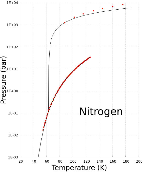
FIGURE 1 P − T phase diagram of Nitrogen. Black solid-line corresponds to prediction of the Non-CEoS reported in this work. Red dots are experimental data [17,26,27].
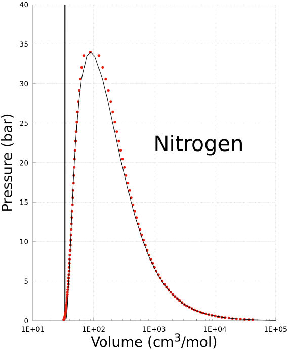
FIGURE 2 P − V phase diagram of Nitrogen. Black solid-line corresponds to prediction of the Non-CEoS reported in this work. Red dots are experimental data [27].
Ammonia is another example. In Fig. 3 experimental data is compared with the prediction made with the Non-CEoS in a P − T phase diagram. The prediction from the Non-CEoS includes solid-liquid and solid-vapor coexistence states that cubic equations of state can not predict, and is in agreement with the experimental data.

FIGURE 3 P − T phase diagram of Ammonia. Black solid-line corresponds to prediction of the Non-CEoS reported in this work. Red dots are experimental data [28,29].
Thus, at least in these three examples the prediction capability of the Non-CEoS is demonstrated, but this feature is applicable to all substances in the database. A special case is that of water, that will be discussed in the following section.
4.2. The water case
Water is a special case of substance. Water molecules can be organized in several clusters with different geometries mainly because their dipole moment. Thus, there are several triple points at its phase diagram, and define several ice types. In particular, the ice-I has a solid-liquid boundary with negative slope so that the melting point decreases with pressure. This feature is due to the dipole-dipole interactions which are highly anisotropic.
On the other hand, the last term in Eq. (1a) for the NonCEoS corresponds to very short-range interactions between the molecules, and the solid phase is formed with these interactions. However, the last term in Eq. (1a) must correspond to an isotropic potential. Under this conjecture, the resulting melting curve of ice-I, which is predicted with the Non-CEoS, must not describe a negative slope because the equation of state is isotropic. The phase diagram of water is showed at Fig. 4. The black solid-line at Fig. 4 corresponds to the prediction of Non-CEoS in this work, while the red dashed-line corresponds to the International Association for the Properties of Water and Steam (IAPWS) data [30,31]. Clearly, the resulting phase diagram does not capture the negative slope of the melting curve of ice-I. But, for the rest of the melting curve, the resulting phase diagram is in agreement with the IAPWS data for high temperatures. In the same Fig. 4, the agreement between the vaporization curve predicted with the Non-CEoS and the IAPWS data is evident. Moreover, there are a small deviations of the pressure near to the triple point and below to it, namely, the sublimation curve. In these cases, the small deviations are magnified by the log scale.
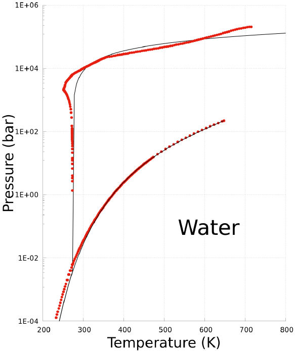
FIGURE 4 P −T phase diagram of water. Black solid-line corresponds to prediction of the Non-CEoS reported in this work. Red dashed-line corresponds to IAPWS data [30,31].
The fact that the melting and triple points of water are too close is well known. The resulting values of the pressure, the molar volume, and the temperature computed with NonCEoS at both points are in Table III. In particular, the value of the molar volume of the saturated solid at the melting point and the triple point are extremely close to each other. In fact, both numerical values at Table III differ at the last digits between parentheses, and those digits are located at the eighth to ninth decimal positions. In other words, the pressure is sensitive to the value of the molar volume of the solid phase because there are significant changes of the value of the pressure with a extremely small changes on the molar volume. In spite of the above fact, the Non-CEoS is capable to distinguish the melting point from the triple point (see Table III).
TABLE III Water properties.
| Results | References | Error | |
| Critical point | |||
| Pressure | 220.0bar | 220.64bar | -0.29% |
| Molar volume | 55.9472cm3/mol | 55.947cm3/mol | 0.00% |
| Temperature | 647.096Kelvin | 647.1Kelvin | 0.00% |
| Boiling point | |||
| Pressure | 1.01325bar | 1.01325bar | 0.00% |
| Molar volume(s) | 23.4162cm3/mol | ||
| Molar volume(v) | 30328.0cm3/mol | ||
| Temperature | 373.151Kelvin | 373.15Kelvin | 0.00% |
| Melting point | |||
| Pressure | 1.01325bar | 1.01325bar | 0.00% |
| Molar volume(s) | 22.5297767(70)cm3/mol | ||
| Molar volume(l) | 22.9448(30)cm3/mol | ||
| Temperature | 273.16(57)Kelvin | 273.15Kelvin | 0.01% |
| Triple point | |||
| Pressure | 0.0036256bar | 0.0061173bar | -40.7% |
| Molar volume(s) | 22.5297767(58)cm3/mol | ||
| Molar volume(l) | 22.9448(32)cm3/mol | ||
| Molar volume(v) | 6.26586×106 cm3/mol | ||
| Temperature | 273.16(25)Kelvin | 273.16Kelvin | 0.00% |
(s): Saturated solid; (l): Saturated liquid; (v): Saturated vapor.
5. Conclusions
A Non-CEoS was constructed for several substances, and the pure substance parameters are reported at Table II. The analytical expression of Non-CEoS is defined through parameters {b,c,d,e,f,λ,ε}. In this work, the procedure to obtain these parameters using experimental data was explained. The experimental data required to define the Non-CEoS are: critical pressure P c , critical molar volume v c , and critical temperature T c , acentric factor ω, boiling point temperature T b , and the temperature T t at the triple point; all of them are in Table I.
The Non-CEoS, described in Eqs. (1a)-(1d), predicts the solid-liquid, solid-vapor, and liquid-vapor phase coexistences of pure substances. This feature was demonstrated with the nitrogen, ammonia, and water cases, and is also valid for all the substances in Table I. Considering the example cases, a good agreement between the resulting phase diagrams predicted with the Non-CEoS and the experimental data was observed.
The adjustment of the values calculated with the NonCEoS for the critical point, acentric factor, boiling temperature, and triple point temperature with respect to their experimental values, is observed through the error reported in the database (see Table II). For almost all substances in the database the numerical relative deviation is less than 1%.
The results for the solid-liquid coexistence (compared with experimental data) enable us to confirm that the last term in Eq. (1a) is related to short-range interactions between the molecules in the fluid. This is manifested by a big value of exponent (in this work ν = 12). Thus, this term modifies the cubic equation only in a region defined by a small neighborhood close to the exclusion volume. As a consequence, the pressure of the saturated solid phase is highly sensitive to the volume value, and therefore, the slope of the melting curve is very pronounced. Another implication of this fact is manifested on the calculation of the melting point temperature, because the difference between the melting point temperature and the triple point temperature is less than 1 Kelvin, as in the water case in Table III.

