


 nueva página del texto (beta)
 Inglés (pdf)
 Artículo en XML
 Referencias del artículo
 Enviar artículo por email
 Citado por SciELO
  Similares en
SciELO
Similares en
SciELO 
 Permalink
1. Introduction
Quantum groups and quantum algebras have attracted much attention of physicists and mathematicians recently. There had been a great deal of interest in this field, especially after the introduction of the q-deformed harmonic oscillator. Quantum groups and quantum algebras have found unexpected applications in theoretical physics [1]. From the mathematical point of view they are q−deformations of universal enveloping algebras of the corresponding Lie algebras, being also concrete examples of Hopf algebras. When the deformation parameter q is set equal to 1, we recover usual Lie algebras. The realization of the quantum algebra SU(2) in terms of the q-analogue of the quantum harmonic oscillator [2, 3] has initiated much work on this topic [4-6]. Biedenharn and Macfarlane [2,3] have studied the q-deformed harmonic oscillator based on an algebra of q-deformed creation and annihilation operators. They have found the spectrum and eigenvalues of such a harmonic oscillator under the assumption that there is a state with a lowest energy eigenvalue.
In the last few years, q−deformations have become a topic of great interest and various applications have been found in several branches of physics, such as q−deformation of the harmonic oscillator, q−deformed Morse oscillator, classical and quantum q−deformed physical systems, Jaynes-Cummings model and the deformed-oscillator algebra, q−deformed supersymmetric quantum mechanics, for some modified q-deformed potentials, on the thermostatistic properties of a q-deformed ideal Fermi gas, q−deformed Tamm-Dancoff oscillators, q-deformed fermionic oscillator algebra, and thermodynamics, and finally on the fermionic q−deformation and its connection to thermal effective mass of a quasiparticle (see Ref. [7] and references therein).
The displacement of charge through a dielectric material plays an essential role in a wide variety of electronics or imaging devices. A detailed understanding on the process dynamics can provide considerable information concerning the material’s electronic structure. Experimentally, the time rate of displacement of charge, as well as the efficiency of their generation by light or energetic electrons, has been studied using a time-of-flight technique (for more detail about this technique see Refs. [8-11]).
In TOF measurements, a semiconductor thin film is sandwiched between electrodes and at least one of the electrodes is blocking for carrier injection, and through one of the electrodes a short light pulse of strongly absorbed light excites a thin layer of electron-hole pairs. Depending on the polarity of an applied electric field, either holes or electrons are drawn into the bulk. The carriers reach the opposite electrode in a transit time t r , which is easily identified as either a rapid drop in the transient photo-current in case of nondispersive transport or an inflection point in the double logarithmic plot of the transient photo-current in case of dispersive transport. In addition, a dispersive transport is the result of a broad distribution of release times from localized states. This distribution can arise from a sped of binding energies of traps (MT) or from a distribution of hopping rates among iso-energetic localized states. If it arises from hopping, dispersion occurs only in the presence of an electric field. This is because, as pointed out by Schmidlin and Kastner [8,9], the occupation of the various states cannot change with time in the absence of the field since they are already in thermal equilibrium. When the field is turned on, the states are no longer in equilibrium because their energies are altered, and the dispersion begins. For these reasons, the (TOF) measurement method is a useful technique to evaluate transit time for mobile objects and is often used for investigating the charge carrier transport properties in various condensed materials including inorganic and organic semiconductors. The resulting transient current provides us with not only transit time but also information on dynamical events in charge transport through a sample, such as trapping and releasing of carriers in trap states, carrier diffusion, and percolation.
Schmidlin and Noolandi [10,11] proposed the multipletrapping model (MTM) to describe such dynamic events of charge carriers in a sample with conventional sets of coupled kinetic equations for trapping and thermally releasing rates. This method can reproduce the experimental current signal I (t), if a subset of trapping- and releasing-rate parameters are suitably assumed. Thus, the MTM has been widely and successfully used to analyze transient-current decays not only in inorganic but also in various organic semiconductors. The films include amorphous inorganic or organic semiconductors, with adequate supposition of trapping and releasing parameters in the form of continuous distribution of trap states such as an exponential distribution e −E/kBT , a Gaussian distribution or other shapes of trap distribution. However, this method is applicable only when a shape of the trap distribution is appropriately taken to describe the distribution of localized states playing the major role in trapping events [12].
Naito et al., [13-16] have proposed a spectroscopic method for extracting localized-state distributions from an analysis of transient photo-current measured with transient photo-conductivity or the TOF technique using the Laplace transform, within a multiple-trapping framework and by means of appropriate approximations. Using a method based on the Laplace transform method, has a number of advantages when compared with other methods: (i) the localizedstate distributions in materials exhibiting either nondispersive or dispersive transport are extracted, the analysis is computationally straightforward and rapid, and (ii) the localizedstate distributions are extracted from both pre- and postmonomolecular recombination regimes of transient photoconductivity or from both pre- and post-transit time regimes of TOF photo-current transient, which hence leads to the measurement of a wider range of localized-state distributions.
After all this brief description, we are ready to expose the objectives of our paper: encouraged by the fact that the qdeformed formalism has interesting and promising results in physics (see [17] and references therein), we are in measure to do the following tasks (i) rewriting the (MTM) equations in the framework of the q-deformed formalism, and (ii) then construct theoretically the deformed simulated currents: this construction is given by using a program based on the Padé approximation. This program allows us to obtain these currents [18]. In all calculations, the electric field has the following form [19,20]
So far, the MTM equations with this type of the electric field have not been studied in the literature. From Eq. (1), we notice the following: (i) ξ (x) = −dV /dx can also be considered as an external force associated with the potential V (x), (ii) k 2 = 0 corresponds to the important case of external constant force, and (iii) finally k 1 = 0, corresponds to the socalled Uhlenbeck-Ornstein process. The Uhlenbeck-Ornstein process describes the stochastic evolution of particles under the influence of friction. This process is stationary, Gaussian, and Markov, which makes it a good candidate to represent stationary random noise [19,20].
Thus, in order to realize the goals of this paper, we first study the usual case, i.e., without introducing any deformation. Then, we consider and discuss the problem in the framework of q-calculus.
This paper is organized as follows: after an introduction, we treat analytically the TOF measurements with the multiple trapping model (MTM) in Sec. 2. Then, in Sec. 3 we extend and study the (MTM) in the framework of q-calculus formalism. The paper is ended by a conclusion provided in Sec. 4.
2. Analytical treatment of the tof measurements with the multiple trapping model (MTM)
2.1 Solutions of (MTM) equations via the Laplace transform (LT)
The continuity equations which define the multiple-trapping problem are first formulated in the familiar context of an electronic carrier moving through extended states with localized gap states acting as trays. It is then shown that the same equations apply to any mobile entity which simply stops and starts at random from a distribution of resting places. The probability of generation per unit volume per unit time is denoted g ν (x,t) = p 0 δ (t)δ (x). Subsequent to generation, the hole drifts (under the influence of an x-directed electrostatic force eF, where e is the fundamental electronic charge) toward a substrate at x = L. At a point x, where the hole may be captured and released from a trap, the appropriate continuity equations may be written [9-11]
where x is the distance from the illuminated surface, p(x,t) and p i (x,t) are the local populations of the transport states and trap i, and p 0 is the injected free carrier density per the unit area. The delta functions define the initial condition for (TOF) experiment. The local flux of mobile holes may be written
where ξ (x) is the electric field. The simplest form that can be given for this function is
Now, using Eqs. (4) and (5), we obtain
The delta function in Eq. (6) defines the optical excitation for the TOF experiment. These equations can be solved using Laplace transforms under the initial and boundary conditions of p(x,0) = 0andp(0,t) = 0.
The Laplace transform of p(x,t) is defined as
0 Using this definition, we obtain
with
Now, the general solutions of (9) are
For a TOF experiment, the photo-current is given by [9-11]
which e is the charge of a carrier: this equation is transformed into
with k 1 = µ 0 F , 0 < k 2 < k 1 /L = µ 0 F/L, and t 0 = L/k 1 is the transit time of untrapped carrier. With the following substitutions α = k 2 L/k 1 < 1, Eq. (13) is rewritten, with the new parameter α, as follows
where the parameter α contains the influence of both parameters k 1 and k 2.
In the limit case, where k 2 → 0 (case of external constant force), and by using that α x = e xlna , we have
and consequently, both (11) and (14) become
Therefore, we recover the usual form of charges and currents [10,11].
2.2. Results and discussion
In order to construct a current numerically, we proceeded with the following steps: as well-known, the inverse Laplace of a function is given by
which I (s) is defined by Eq. (13). When we use the following change of variables, z = st, and dz = sdt, the integral becomes
To calculate the last integral we use the method exposed in [18]. So, according to Eq. (19), the computed current can be obtained as follows: (i) Firstly, we express the function e z in its Pade approximation expansion: Padé approximation of a function is somewhat similar to a Taylor series, except that the expansion is a ratio of two polynomials. (ii) Secondly, we apply the Residue theorem to obtain the desirable function, i.e., the computed current I(t). Thus, in our case, we calculated the inverse Laplace transform numerically, using the Padé approximation (a rational approximation with polynomials of 8-degree). The physical quantities used in the computation were σν th = 10−7 cm3/s, ν = 1012 s−1, T = 300 K, and g (E) = 1021e−(E/kbT0) with k b = 8.625 × 10⁻⁵ eVK−1 is the Boltzmann constant.
Now, we are ready to show and discuss all the results found by the program used to obtain our simulated currents.
Figure 1 shows the normalized photo-currents vs times in the (log-log) scale for different values of parameters k 1 and k 2 or α = k 2 L/k 1.

FIGURE 1 a) For different values of T 0. b) For fixed α and T 0 < T. c) For different values of α where T 0 > T. d) For different values of α where T 0 < T. e) For fixed value of α and T 0 > T. f) For fixed value of α and different values of Field. The normalized photo-currents vs times in the temperature T = 300 K.
In Fig. 1a), we present the normalized currents for fixed value α = 0.5 and for various characteristic temperatures T 0. It is clearly seen that the transient photo-current decreases with time. For non-dispersive transport, with T 0 = 250 K, the transit time can be obtained at the intersection of the transient photo-current with the time-axis. Similar results are obtained for dispersive transient photo-current. Now, for all the temperatures T 0 < 300 K, as shown in Fig. 1b), we observe that all the curves have typically the same behavior in preand post-transient regime.
Figures 1c) and 1d) depict the behavior of the currents in both T < T 0 and T > T 0 interval of temperatures, and that for various values of α: in this case, we specified two regimes: in the region where T 0 > T, all the curves in both pre- and post transient regime are the same. In the other hand, where T 0 < T, these curves show that the form of the currents in the pre-transient regime are identical contrarily to the case of the post-regime where the difference becomes clear.
Figures 1e) and 1f) illustrate the current transients at various values of applied electric fields for a fixed value of the parameter α. An interesting observation pointed out in Fig. 1f) is that the inflection point is affected by the applied field. The transit time is much shorter than the mono-molecular recombination lifetime. In this case, the inflection points shift toward a shorter time regime by increasing the applied electric field. This means that the inflection point is due to the transit time. From these results, we can experimentally distinguish whether or not the inflection point is the charge carrier transit time: if the inflection point becomes shorter with an applied electric field, then the inflection point is charge carrier transit time.
3. Solutions of a multiple-trapping equations in the framework of q-deformed formalism
We aim in this section to discuss in the frame work of q-calculus the problem described by continuity equations Eqs. (2) and (3). We present in the Appendix A a survey of q-calculus algebraic properties.
3.1. q-derivative and q-integral
The q-derivative, in the framework of the q-calculus formalism, is defined as
The development of this framework of q-deformations inspired the definition of deformed expressions for the logarithm and exponential functions, namely, the q-logarithm and the q-exponential (q-exponential Tsallis [19]), first proposed as
where [A]+ ≡ max{A;0}(1 + (1 − q)x > 0). Both equations can be rewritten as
where both equations are restricted to the following condition 1 + (1 − q)x 6= 0. Also, we have the following well-known relations:
where (see Appendix A)
The q-derivative obeys
• Leibniz rule
• the chain rule
The corresponding q-integral is given by
with
3.2. Solutions
Now, when introducing the q-derivative formula, Eqs. (2) and (3) become
with
and here
Using Eqs. (34) and (35), Eq. (32) is transformed into
By using the Laplace transform method, Eq. (36) reads as
The solutions of Eq. (37) are
In the limit case, where q →,1, we recover the Eq. (16).
The q-deformed Laplace of current has the following form
Putting Eq. (38) into Eq. (39) leads to
The general solution of this integral is
where
with
and 2 F 1 is the hypergeometric function.
In this stage, an important remark can be made: following these equations, we observe that obtaining the exact form of currents is a very hard task. To overcome this problem, seeking simplicity, we will concentrate only on the case where k 2 = 0 (constant electric field). So, the form of the currents I (s) as well as the charges p(x,s) reduced to the following relations:
with
In the limit case, where e q (x) q→1 = exp(x), we recover the desired relations of currents and charges as described by Eqs. (16) and (17).
Now, before commenting on our results, we can note that the linear form of the electric field can be considered as a deformation whose parameter is k 2 /k 1. Starting with the following equation
Setting −(k 2 /k 1) = 1 − q or q = 1 + (k 2 /k 1), Eq. (50) is transformed into
Thus, the form of the current is changed to
or
In the limit case, where k 2 → 0 (the constant electric field), we recover well Eqs. (11) and (13).
Thus, the linear form of the electric field chosen here Eq. (1) can be considered as a deformation with the parameter α. This remark allows us to try to study the (MTM) equations in the framework of q-calculus formalism.
Now, in the framework of the q-calculus formalism, we are ready to discuss the results concerning calculation of normalized currents in different choices of both T 0 and F. All the results are obtained by using the same program as above [18].
3.3. Results and discussions
Figure 2, obtained using the program developed in [18], shows the normalized currents vs time for various values of the parameter q in both regions of the temperatures T > T 0 and T < T 0. In all the curves, the value of the electric field is fixed.

FIGURA 2 a) For different values of q and with T0 < T. b) For different values of q and with T 0 > T. c) For fixed value of q and in both regions T < T 0 and T > T 0. The q-deformed normalized photo-currents vs times.
Figure 2a) depicts the variation of the current vs time, where T 0 = 290 K and F = 4 × 10⁴ Vcm−1. Two remarks, in both intervals of temperatures, can be made here:
In the case where T 0 < T
all the curves in the per-transient regime coincide whatever the value q, contrarily in the posttransient regime where the difference becomes clear,
the deflection point (transit time t r ), in both preand post-transient regime, increases when q increases until the usul limit when q = 1,
this time, for fixed value of q, decreases when the electric field F increases (see Fig. 3).
Now, in the other case where T 0 > T
As we know, the TOF measurements allow us to calculate a thermally activated drift mobility for both holes and electrons [21-26]. In addition, the transient hole transport at low temperatures T < 180 K obey the stochastic transport formalism, whereas above T ∼ 200 K, it seems following the conventional (Gaussian) transport concepts, evincing a welldefined transit time t r in the TOF signal (see Ref. [23] and references therein). In addition, many authors have reported field-dependent mobility even around room temperatures, in contrast to the other works which indicated constant mobility over the temperatures down to 250 K [23].
The carrier drift mobilities obtained from the transit times t r were extremely low and strongly field-dependent and the transients were obtained under nearly space-charge- limited conditions [21]. Furthermore, although the shapes of the photocurrents above ∼ 200K show dispersion which diminishes with increasing temperature the TOF drift mobility,
displays no thickness dependence [23, 24]. Note here that the time transit t r is easily identified as an inflection point in the double logarithmic plot of the simulated transient photocurrents. In Ref. [21], Gill proposed that the observed field and temperature dependences can be incorporated into an empirical relation for the hole or electron mobility of the form
where µ 0 is the zero-field drift mobility and β is the wellknow the Poole-Frankel coefficient.
After this brief discussion about the drift mobility, our principal goal, is to study the influence of the parameter q on the drift mobility. In addition, the Poole-Frankel coefficient will be obtained, for different values of q, from Eq. (55). To do this, we determine firstly the times t r from all the curves of our simulated photocurrents, and this for different applied electric field F (see Fig. 3). Using Eq. (55), we easily calculate the drift mobility vs the electric field by varying the values of the temperature T and the parameter q (see Fig. 4).
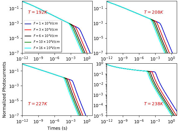
FIGURE 3 The normalized photo-currents vs times for different values of electric field: here q = 0.2.
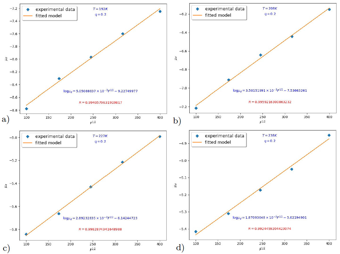
FIGURE 4 a)T = 192 K. b)T = 208 K. c) T = 227 K. d) T = 238 K. Temperature dependence of the drift mobility with electric field for q = 0.2: experiment data means the currents plotted in Fig. 3.
In Fig. 3, we show the normalized currents versus a time where q = 0.2. The same thing can be done for specific choices such as q = 0.5,0.7and0.9. After choosing the time t r , for each values of temperatures T = 192, 208, 227, and 238 K, we calculate the values of the drift mobility, for each value of q.
In order to verify the validity of Eq. (55), we have constructed Fig. 4. This Figure shows the field dependence of the drift mobility represented as logµ versus F 1/2 . It can be seen that the drift mobility seems to follow Eq. (55).
These Figures show a linear form of logµ d versus F 1/2 for different values of the parameter q. The slopes of these fit allow us to determine the values of the Poole-Frenkel coefficient β pf . An important remark about the Poole-Frenkel model can be made here. The field and temperature dependence expressed in Eq. (55) is similar to the observed behavior of the conductivity in some insulating solids. These results have been explained using the Poole-Frenkel mode in which the Coulomb potential near a charged localized state is modified by the applied field so as to increase the free-carrier density at high fields. More precisely, the essence the PooleFrenkel effect is the field-assisted lowering of the coulombic potential barrier between carriers at impurity levels and the edge of the conduction or valence bands. When a carrier is trapped at a center, it is unable to contribute to the conductivity until it overcomes a potential barrier and is promoted into one of the free bands. In the presence of a high electric field the potential is reduced by an amount eFx where e is the electronic charge, F is the applied field and x is the distance from the center. Now, by assuming trap-controlled drift mobility, the Poole-Frenkel model can be applied to driftmobility results [22,27,28].
The theoretical values β pf are determined by the following relation [22-26]
where ε 0 is the permittivity of free space, ε r is the relative permittivity of the dielectric and e is the electronic charge.
The values of the coefficient β PF and the relative dielectric constants ε r are shown in Table I, for L = 50 µm at various temperatures and parameter T and q respectively. The range of the temperatures are T = 192 K, 208 K, 227 K, and 238 K, where the characteristic temperature T 0 = 300 K.
TABLE I The estimate of the Poole-Frankel coefficients βPF at some values of the temperatures and the parameter q
| (a) q = 0:2 | (b) q = 0:5 | ||||
| T (K) | Βpf(10-5eV(Vm-1)-1/2) | ϵr | T (K) | Βpf(10-5eV(Vm-1)-1/2) | ϵr |
| 192 | 2.55 | 9 | 192 | 2.55 | 8.63 |
| 208 | 2.4 | 10 | 208 | 2.40 | 10.81 |
| 227 | 2.3 | 11 | 227 | 2.30 | 10.64 |
| 238 | 2.35 | 10.5 | 238 | 2.35 | 11.17 |
| (c) q = 0.7 | (d) q = 0.9 | ||||
| 192 | 2.53 | 9 | 192 | 2.57 | 8.81 |
| 208 | 2.43 | 9.86 | 208 | 2.35 | 10.55 |
| 227 | 2.15 | 12.53 | 227 | 2.14 | 12.70 |
| 238 | 2.21 | 11.87 | 238 | 2.12 | 13 |
From this table, we can see that [29]
• the estimate values of β PF are about of 10−5 , and are approximatively the same as those obtained in the literature (see Table II). In addition, these values agree remarkably with that calculated for the one-dimensional case in [22-24],
• The values of relative dielectric constant for PooleFrenkel coefficient are in the range 4.8-12.
Finally, an important point can be made about the parameter of deformation q which is the central quantity of qcalculus formalism: According to the recent works [30-33], this parameter can play a role of fitting the experimental results. To better understand this, we can mention the work of Guha and Prasanta [34]: the authors have applied the theory of q-deformed (Tsallis statistics) to describe specific heat of solid by using the Einsteins model which is well-known in the theory of physics solid state. As we know, in the ordinary physics of solid state, the Einstein model of the solid predicts the heat capacity accurately at high temperatures which is equivalent to Dulong-Petit law. Nevertheless, contrarily to the Debye model, the heat capacity noticeably deviates from experimental values at low temperatures. In this context, the authors have been successful in solving this disagreement which appears at low temperature. They have studied the temperature fluctuation effect via the fluctuation in the deformation parameter q. As a result, they found that, at low temperature, the Einstein curve of the specific heat in the Tsallis scenario exactly lies on the experimental data points and matches with the Debye’s curve. In addition, they claim that a unique value of the Einstein temperature θ E , along with a temperature-dependent deformation parameter q (T), can describe the phenomenon of specific heat of solid i.e. the theory is equivalent to Debye’s theory with a temperature-dependent θD.
In this direction, we can better understand the principal aim of our contribution to this paper. Despite the nonexistence of direct experimental verification of our model, we can claim that our approach, i.e., the introduction of the q-calculus formalism, can improve our understanding on the physical behavior of charge carriers in amorphous semiconductors.
4. Conclusion
In this paper, we analyze multiple-trapping model (MTM) for charge carrier transport from time-of-flight transient (TOF) photo-current in amorphous semiconductors in the generalized non-extensive scenario (Tsallis statistics). This generalized statistical techniques (in Tsallis statistics q being the deformation parameter) have been applied to a wide range of complex systems. In our case, we have first discussed the solutions of the (MTM) equations with the existence of a linear form of an electrical field. The normalized currents, I (s)/I (0), have been obtained by using a program that we have developed in order to calculate the theoretical currents. With this program, a good agreement between the experimental and theoretical currents have been found (see Ref. [14]). Next, we considered the (MTM) equations in the framework of the q-calculus, the influence of the parameter q in the curves of the current have been well observed. These currents were obtained also by using the same program that has used in the first case. Moreover, we studied the influence of the parameter q of the q-calculus formalism on the drift mobility. It is shown that at low temperatures the drift mobility may be described by an empirical expression with the√ following form µ d = µ 0 e β F/kbT . This form holds too in our case. Finally, the well-known β pf , called Poole-Frankel coefficient, are determined.

