2.1. Scenarios for the generation of cosmic magnetic fields

For magnetic fields at large scales, the key problem is that a seeding mechanism that can account for both scales and strengths of the presently observed fields has not been found. There are two basic scenarios for their generation: they could be either primordial (generated before the recombination epoch) or produced during processes associated with structure formation, and these possibilities are not mutually exclusive. The growing observational evidence for the presence of magnetic fields at all astrophysical scales strengthens the idea of the primordial origin of cosmic magnetism. This possibility implies a further difficulty besides the one of finding the generation machinery: mechanisms for their preservation and amplification must also be defined.

A series of mechanisms for early magnetogenesis have been proposed [²³-²⁶] (see also [²⁷] for a review), most of them based on cosmological phase transitions that can provide suitable conditions for their generation, such as charge separation (battery mechanism), turbulence and departure from equilibrium. However, none of them are problem-free, being the scale the principal drawback, due to causality reasons.

The earliest epoch magnetic fields could have been born at super-horizon scales is inflation, relying on the fact they can be created by the same mechanism that generated density fluctuations, i.e., quantum fluctuations in the Maxwell field, excited inside the horizon, are expected to freezeout as classical electromagnetic waves once they cross the Hubble radius. These initially static electric and magnetic fields can subsequently lead to current supported magnetic fields, once the excited modes reenter the horizon. Nevertheless, fluctuations that survive a period of de Sitter expansion are typically too weak to match the present observations, as long as magnetic fields decay adiabatically with the universe expansion. To avoid this suppression, some options have been presented: in [²³,²⁸] some mechanisms that break conformal invariance of electromagnetism are introduced (see, however [²⁹]), and in [³⁰], it is shown that the magneto-geometrical interaction can change the evolution of large scale magnetic fields, in perturbed Friedman-Lemaıtre-Robertson-Walker cosmologies with open spatial curvature. On another hand, since superhorizon-sized fields are not governed by causal physics, in [³¹], this adiabatical suppression has been questioned. Anyway, it has been pointed out that an obstacle to inflationary magnetogenesis might be the so-called back reaction problem [³²], which consists of the fact that the generation of magnetic fields during inflation increases the electromagnetic energy density, which can eventually dominate over the inflaton energy.

Another possibility for generating primordial magnetic fields (PMF) is to resort to the properties of the vacuum in non-Abelian gauge theories, where it can present a ferromagnet-like configuration (Savvidy vacuum). In [³³,³⁴], it has been shown that this non-zero magnetic field configuration is present even at high temperatures. The formation of this non-trivial vacuum state at Grand Unification Theories (GUT) scales can give rise to a Maxwell magnetic field imprinted on the comoving plasma.

To gain some insight into the features and strengths of PMF, one can resort to cosmic observational events. The imprint of PMF has been searched in the cosmic background radiation (CMB) (see e.g. [³⁵] and references therein), in the nucleosyhthesis process (a detailed review can be found in [³⁶]), in structure formation [³⁷] and the primordial gravitational waves spectrum [³⁸]. Limits obtained from different events, typically involve different coherence scales, established by the Hubble radius at that epoch. The reported strengths (B ₀) are usually scaled to present values assuming adiabatic evolution. Another assumption that must be done is the shape of the power-spectrum, P _B (k), which is usually considered to depend on k as a simple power-law function on large scales: P _B (k) ∝ k ^nB . In this case, PMF are completely described by two parameters: the spectral index, n _B (an important parameter for the discrimination between models of magnetogenesis), and the root-mean-square of the field smoothed over some length scale. Alternatively, bounds on the total magnetic field energy density are found.

From nucleosynthesis, an upper bound of B ₀ ≤ 3×10⁻⁷ G, at length scales of the order of the Hubble horizon size at Big Bang Nucleosynthesis (BBN) time (which today corresponds approximately to 100 pc^iv [³⁹]) or an updated value hB ₀i ≤ 1.5×10⁻⁶ G (related to the contribution to the local field amplitude B from all wavelengths) [⁴⁰] can be found. From the large-scale structure formation process, the imprints of PMF can be searched through the thermal-SZ effect, leading to the bound B ₀ ∼ 10⁻⁸ G (see e.g. [⁴¹,⁴²] and references therein), the Lyman-alpha forest: B ₀ ∼ 10⁻⁹ G, at scales 1 Mpc for a range of near scale-invariant models, corresponding to magnetic field power spectrum index n ' −3 [⁴³], or the matter power spectrum, leading to the bound of B ₀ ∼ 1.5−4.5×10⁻⁹ G and n _B ∈ [−3,−1.5], considering the total magnetic field energy density [⁴⁴].

Stringent constraints emerge from considering different aspects of the interaction of PMF with the CMB, as well as different features and scales of these cosmic fields (see for instance [⁴⁵,⁴⁶], and references therein). Constraints have been derived using the CMB temperature and polarization power spectra [⁴⁷-⁵⁰], Faraday rotation [⁵¹-⁵³], cosmic birefringence, and studying its non-Gaussian correlations, considering the bispectrum [⁵⁴,⁵⁵] as well as the trispectrum [⁵⁶]. The upper bounds that are established are between a few and a tenth of nano Gauss. Considering, in particular the bounds, obtained from Planck data [⁴⁷], the most stringent constraints for B ₁ Mpc are in the range 1-4 nano Gauss.

There are also more indirect observational imprints, as the effects of PMF on cosmological phase transitions, that have been extensively studied, including the electroweak phase transition [⁵⁷-⁶²], with particular emphasis on the baryogenesis process (See [⁶³] for a review; see also [⁶⁴]), or the possible supersymmetric phase transitions [⁶⁵-⁶⁷].

Regarding compact objects, the two commonly considered mechanisms for magnetic field production are the fossil field hypothesis and the turbulent dynamos theory [⁶⁸]. According to the fossil field hypothesis, stars’ magnetic fields have their origins in the magnetic field available in the hosting galaxy at the moment of star formation. Or in the case of a compact object, in the magnetic field of the progenitor star. The lines of forces of these fields are assumed to be frozen in the plasma, with the magnetic field increasing as the matter is compressed [⁶⁹]. The main support to this hypothesis in the case of compact objects is the fact that the observed magnetic flux of some CO progenitors equals the one typically found in these stars [¹⁴,⁷⁰,⁷¹]. However, there is not a clear physical reason why the magnetic field should remain frozen during the CO formation and, also, the fossil field hypothesis does not explain the wide variations of the magnetic fields of different stars nor the higher values of the field attained in magnetars [⁷¹,⁷²]. In this way, even if the fossil field hypothesis is accepted as being behind the magnetic field origin, some kind of amplification is required. The dynamo mechanism consists in the generation of a magnetic field in an electrically neutral conductive fluid from currents circulating in it. These currents can find their origin in some battery mechanism, that relies on the fact that, in a charge-neutral universe, positively and negatively charged particles, having different masses, have different mobility in regions with pressure and temperature gradients (see, e.g., [⁶⁸]). Again, this mechanism usually produces seed fields much weaker than the observed ones. Amplification is usually thought to be done by dynamo-like mechanisms [⁶⁸], that keep converting kinetic energy into magnetic one, thanks to the internal inhomogeneities of the star. However, despite the many existing dynamo models, all of them are incapable of explaining all the observations, in such a way that the problem remains open [⁶⁹,⁷¹,⁷³].

Besides dynamo theories, another magnetic field amplification mechanism has begun to be considered recently: self-magnetization [⁶⁹,⁷⁴,⁷⁵]. Since all elementary particles have an intrinsic magnetic moment, and this magnetic moment determines microscopic magnetic fields, the alignment of these micro magnetic fields may generate large scale fields. The micro field alignment, or self-magnetization, may be due to spin-spin ferroelectric-like interactions [⁶⁸], or, in the case of bosonic matter, due to a phenomenon known as Bose-Einstein ferromagnetism [⁷⁶]. Actually, in [⁷⁷], Bose-Einstein ferromagnetism was proved to be enough to produce magnetic fields as high as those expected in magnetars.

2.2. Modeling magnetic fields in compact stars

Magnetic fields affect the microphysics as well as the macrophysics, i.e., the observables, of compact objects. At a microscopic scale, the magnetic field can always be considered locally uniform and constant. Although the consequences of the presence of a magnetic field on an specific star model depend on how matter-field interactions are considered, there are two general ways in which the field modifies the physics of the CO. On the one hand, the field changes the interaction energies and the percentage of particles composition, through direct and inverse beta decay. On the other, the magnetic field breaks the SO(3) symmetry of the system causing an anisotropy in the energy-momentum tensor that leads to anisotropic equations of state. This effect is general, independently of what kind of particles is considered.

The microscopic effects of the magnetic field described in the last paragraph have a direct impact on the macrophysics of the CO, causing modifications to the observables. In particular, as the anisotropic EoS are not spherically symmetric, it becomes imperative to go beyond the standard Tolman-Oppenheimer-Volkoff (TOV) equations to obtain the observables of magnetized stars. However, the sources of the magnetic field inside the COs are uncertain, as well as the variations of its geometry and intensity. This lack of knowledge is usually overcome by a set of assumptions that allows getting, at least, some insight into the problem.

Some studies appeal to a simplified solution: to assume that the structure of a strongly magnetized CO can be reasonably described using the standard spherically symmetric TOV structure equations, while the microscopic anisotropy in the pressures is neglected, appealing to a solomonic solution: the use of a unique pressure which is a sort of average of their components [⁷⁸]. Nevertheless, the most common assumption is to consider a constant magnetic field direction and try to solve Einstein equations in an axisymmetric metric. In these approaches, the magnetic field intensity might be either constant or depend on the star inner radius or its baryon density (see e.g. [74,78,79]). In most cases, this dependency is completely ad-hoc, only based on some physical constraints such as the intensity has to decrease from the center to the surface of the star, and reproduce some reasonable magnetic field values at these points [⁷⁸].

In magnetized CO, the scale lengths of variation of the magnetic field from the core to the surface are of the order of their radii, that is tens of kilometers for NS, while the microscopic magnetic scale length^v depends on the magnetic field (lm ∼ 1/eB  ∼ 10-10 km) [⁸⁰], much smaller than the former. This makes reasonable from the Astrophysical point of view the assumption of a constant and uniform magnetic field as the first step of magnetized compact stars modeling. However, there is also the possibility of considering a nonuniform magnetic field and try to derive its intensity and direction by solving the coupled Maxwell-Einstein equations^vi. As a result, a large set of coupled elliptic partial differential equations is obtained, that must be solved through numerical methods [⁷⁸].

Several methods have been developed and made available to the community for attacking this numerical problem. Such is the case, for instance, of the open-source LORENE C++ library^vii for numerical relativity, which allows to use poloidal fields [⁸¹,⁸²]. There is also another public code, as XNS^viii, that supports either the purely toroidal, purely poloidal, or the mixed twisted torus configurations [⁸³,⁸⁴]. Both codes work under the 3+1 formalism^xix [⁸⁵].

Despite their great merit, the nowadays available methods for solving COs with non-uniform magnetic fields still have several drawbacks. The first one is that while the magnetic field intensity is computed through Maxwell equations, the magnetic field geometry is imposed by hand and limited by the numerical methods used for solving Einstein equations [⁸¹]. Secondly, stable configurations of compact objects are sometimes limited by the convergence of the numerical solutions without this being related to any known physical reason. Finally, the existence of currents inside the star is assumed to have magnetic field sources in Maxwell equations; nevertheless, these currents have not an evident direct relationship with the matter described by the EoS.

One of the most discussed effects is whether the magnetic field increases the maximum mass of the star. As we will see below, this is not in general achieved by models with a constant magnetic field; meanwhile, models based on nonuniform magnetic fields are more successful in increasing the star masses, up to 2M_ʘ [¹⁷-¹⁹]. It is also well-known that the inclusion of rotation in COs description increases the maximum masses [⁸⁶], more than the magnetic field presence usually does [⁸⁷]. Rotation produces a flattening at the poles and a blowup in the equatorial direction. Consequently, it enhances deformation and allows stable star configurations with higher masses than their non-rotating counterparts [⁸⁸-⁹¹]. However, in this review, we will not take into account the rotation impact, to deal exclusively with magnetic field effects. Also, since the results regarding magnetized compact objects are very model-dependent, we focus on the simplest shape of the magnetic field, i.e., a constant and uniform configuration. Our principal aim is to show, in the simplest -although not easiest- possible way, how the magnetic field modifies the observables of the stars. Throuhout these pages, two approaches will be presented for deriving structure equations within the axial symmetry imposed by a uniform magnetic field.

4.1 Cylindrical and Spheroidal models of structure equations

An attempt to obtain structure equations for a magnetized compact star was proposed in [101] using an axisymmetric metric which responds better than the spherical one to the symmetry of the problem. In cylindrical coordinates, this metric reads

where now there are three metric coefficients to determine Φ, Λ, and Ψ.

Solving Einstein equations with the anisotropic energy-momentum tensor in Eq. (7), the metric in Eq. (15) and the requirement that the coordinate functions Φ, Λ, and Ψ depend only on the r-coordinate [¹⁰¹], yields four differential equations

that, together with the EoS (P _⊥, E(P _⊥), P _||(Ɛ)), define a system of equations for P _⊥ , P _|| , Ɛ, Φ, Λ, Ψ. The equatorial radius of the star, R _⊥, is computed through the condition P _⊥(R _⊥) = 0. The above system of equations is obtained with the simplification that all magnitudes only depend on the equatorial radius r. The price paid with this approximation is the impossibility to compute the total mass of the CO. However, using the Tolman mass definition [¹⁰²], it is possible to get the mass per unit length

The handicap of the cylindrical model, Eq. (16-17), in getting the total mass of CO, might be overcome by conserving the angular dependence of the metric functions or by the search of other metrics.

In the spirit of this last possibility, in Refs. [¹⁰³-¹⁰⁵], it was shown that a deformed compact object can be described by the metric

where the parameter γ = z/r parametrizes the polar radius, z, in terms of the equatorial one, r.

The metric in Eq. (18), or γ-metric, allows obtaining a set of structure equations that generalize TOV equations to axially symmetric compact objects [¹⁰⁶]

where the functions Ɛ_|| and Ɛ_⊥ are given by the parametric dependence of the energy E on the parallel and perpendicular pressures, (P _|| ,Ɛ) and (P _⊥ ,Ɛ), respectively.

Equations (19) describe the variation of mass and pressures with spatial coordinates, r, and z. To obtain Eq. (19a), the assumption γ ≃ 1 needs to be made. This means that the objects described by Eqs. (19) must not be too far from the spherical shape, since setting γ = 1 in Eq. (18) take us back to Eq. (12).

As for TOV equations, for solving Eqs. (19), one starts from a point in the star center with Ɛ _c = E(r = 0), P _||c = P _||(r = 0) and P _⊥c = P _⊥(r = 0), taken from the EoS, and ends the integration at P _||(Z) = 0 and P _⊥(R) = 0. However, let’s note that, in Eqs. (19), γ is a free parameter that can not be obtained from them. This, of course, contains a difficulty, since it is mandatory to find a way to evaluate γ for solving Eqs. (19).

Because in TOV equations, for a given central energy, a lower central pressure leads to a smaller radius, together with the relation γ = z/r, the authors of [¹⁰⁶] proposed to interpret γ as the ratio between the parallel and perpendicular central pressures. In this way, the ansatz γ = P _||c /P _⊥c connects the geometry of the system with the anisotropy produced by the magnetic field. It implies that the shape of the star is only determined by the anisotropy of the EoS in its center and neglects the fact that the deformation of the star also depends on the inner profiles of the anisotropic pressures. Nonetheless, this model gives reasonable results [¹⁰⁶], and allows to recover TOV equations since, setting B = 0, gives γ = 1.

In the next sections, stellar sequences obtained with Eqs. (14), (16), and (19), are shown for magnetized white dwarfs and quark stars, and the results of using one EoS with different sets of structure equations are compared. Besides the solutions of Eqs. (19) are shown for magnetized BEC stars, along with a related mechanism for magnetic field generation.

5.1. White Dwarfs

White dwarf stars (WDs) are the endpoint of the evolution of stars with masses typically less than 8 solar masses. Their composition is based on Carbon and/or Oxygen. Their densities are in the range of 10⁹ − 10¹¹ g/cm³, their temperatures reach 10⁶−10⁹ K, and they can be modeled as a lattice of non-relativistic ions embedded in a sea of relativistic electrons. The maximum masses of these objects are theoretically limited by the well-known Chandrasekhar mass 1.4 M_ʘ.

Surface magnetic fields in WDs have been measured by several techniques and span from 10⁵ to 10⁹ G. In general, the analysis of the observed data shows that magnetized WDs have larger masses than non-magnetized ones, and models of magnetized WDs have been proposed to describe this observational fact [¹⁰⁷].

In recent years, a debate has emerged, led by Upasana Das and Banibrata Mukhopadhyay, [¹⁰⁸], about whether strong magnetic fields, larger than the Schwinger critical field, could increase the mass of a WD beyond the Chandrasekhar mass. This debate was motivated by the observation of supernovae that appear to be more luminous than expected (e.g., SN 2003fg, SN 2006gz, SN 2007if, SN 2009dc) and whose progenitor should consequently be a WD with mass above the Chandrasekhar limit.

Some of the works that reached Super Chandrasekhar masses require magnetic fields above 10¹³ G. That is unlikely to exist for WDs because they violate relevant microphysics considerations such as inverse β decay and pycnonuclear fusion reactions involved in the calculation of the structure of these objects [¹⁰⁹]. However, the problem was still attractive due to its links with Type Ia Supernova, which are crucial for distance measurements in the Universe [¹¹⁰].

In this context, two works [106,¹¹¹] were developed, revisiting this issue, focusing on the understanding of the role of the magnetic field in the maximum masses of WDs. These studies are based on the anisotropic EoS and its consequences on the structure equations for the axial symmetric metric previously described.

In these models, WDs are sustained by the pressure of the degenerate electron gas and matter, inside the star, must be in stellar equilibrium, so that charge neutrality and baryon number conservation are required. With these considerations, the magnetized WDs EoS are

where Ω is given by Eq. (A.3) of the Appendix, N = −∂Ω/∂µ is the electron particle density and M = −∂Ω/∂B the magnetization. The term Nm _N A/Z, included in

Eq. (20a), accounts for the contribution of ions to the energy density^xii [¹⁵].

The structure of magnetized WDs will be first studied solving independently TOV equations for each pressure. This is equivalent to considering two independent EoS: (Ɛ,P _‖) and (Ɛ,P _⊥). The results are illustrated in Fig. 1 for several values of the magnetic field -10¹¹, 10¹², 10¹³ G- and compared with the non-magnetized case. Note that in the case of (Ɛ,P _⊥), the magnetic field indeed contributes increasing the mass of the star but this occurs only for the less massive stars and not in the regime of maximum masses, which is the one that deals with the issue of the upper bound for WDs masses. As can be observed in this figure, the maximum mass remains bounded by the Chandrasekhar value.

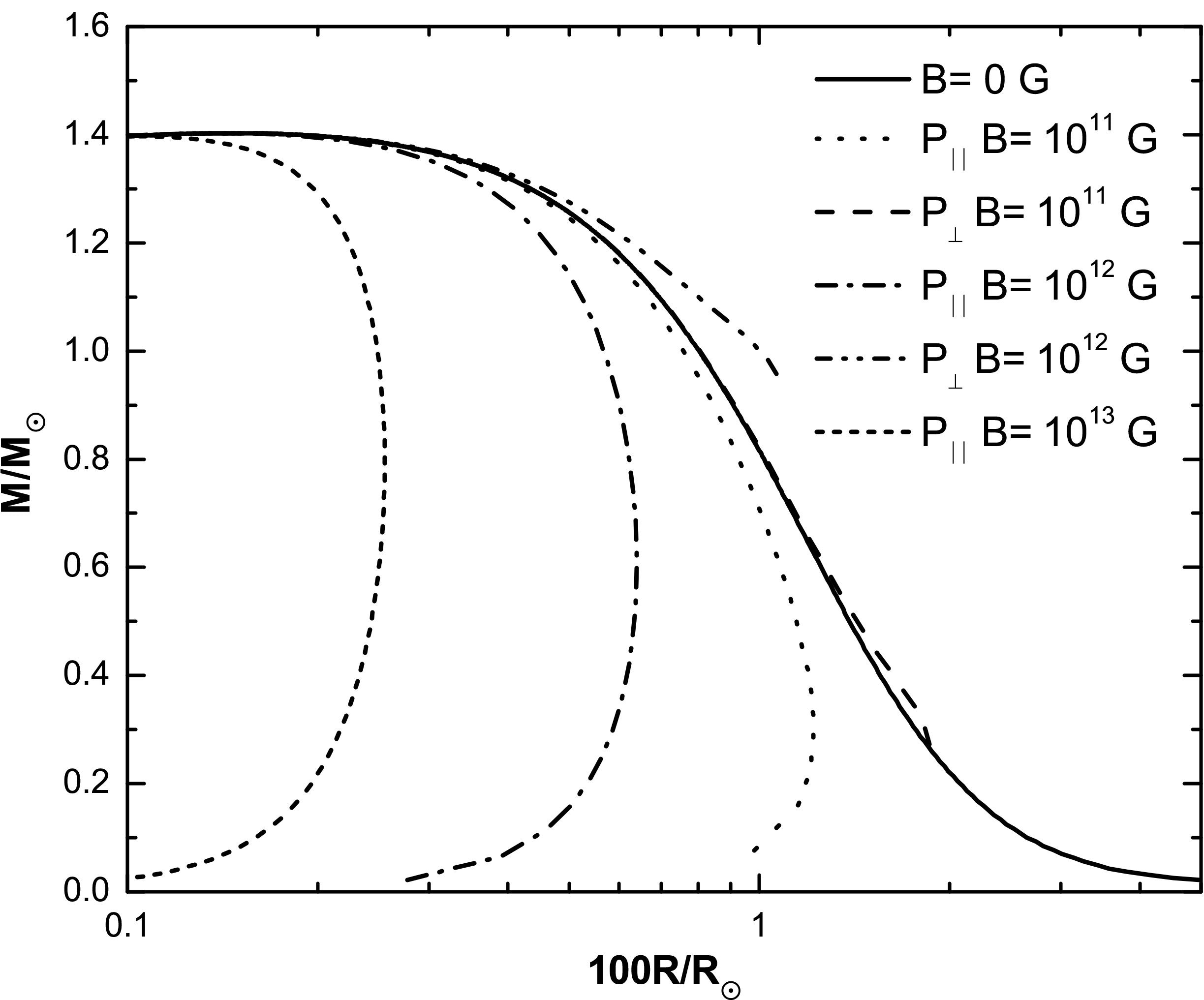
FIGURE 1 Mass-Radius relation for WDs with TOV equations. Two aspects are clearly shown: for a specific mass, a different radius is obtained when considering the parallel and perpendicular pressures, and, independently of the considered pressure and magnetic field strength, masses do not go beyond the Chandrasekhar limit. 

The mass per unit length obtained from Eqs. (16) for WDs is shown in Fig. 2. The magnitude M/M_¯ R _⊥ /R _k, as a function of equatorial radius is plotted. At first glance, Fig. 2 suggests that masses can be greater than in the B = 0 case since values for the magnitude M/M_ʘ R _⊥ /R _‖ are larger. However, this value cannot be associated with the maximum mass for WDs since, because of the indeterminacy of the parallel radius, the total mass cannot be calculated. An interesting result is that, from this study, an upper bound, around 10¹³ G, for the allowed values of the magnetic field for stable configurations of WDs is obtained. Beyond this bound, the metric coefficients diverge, so there are no numerical solutions for the structure equations.

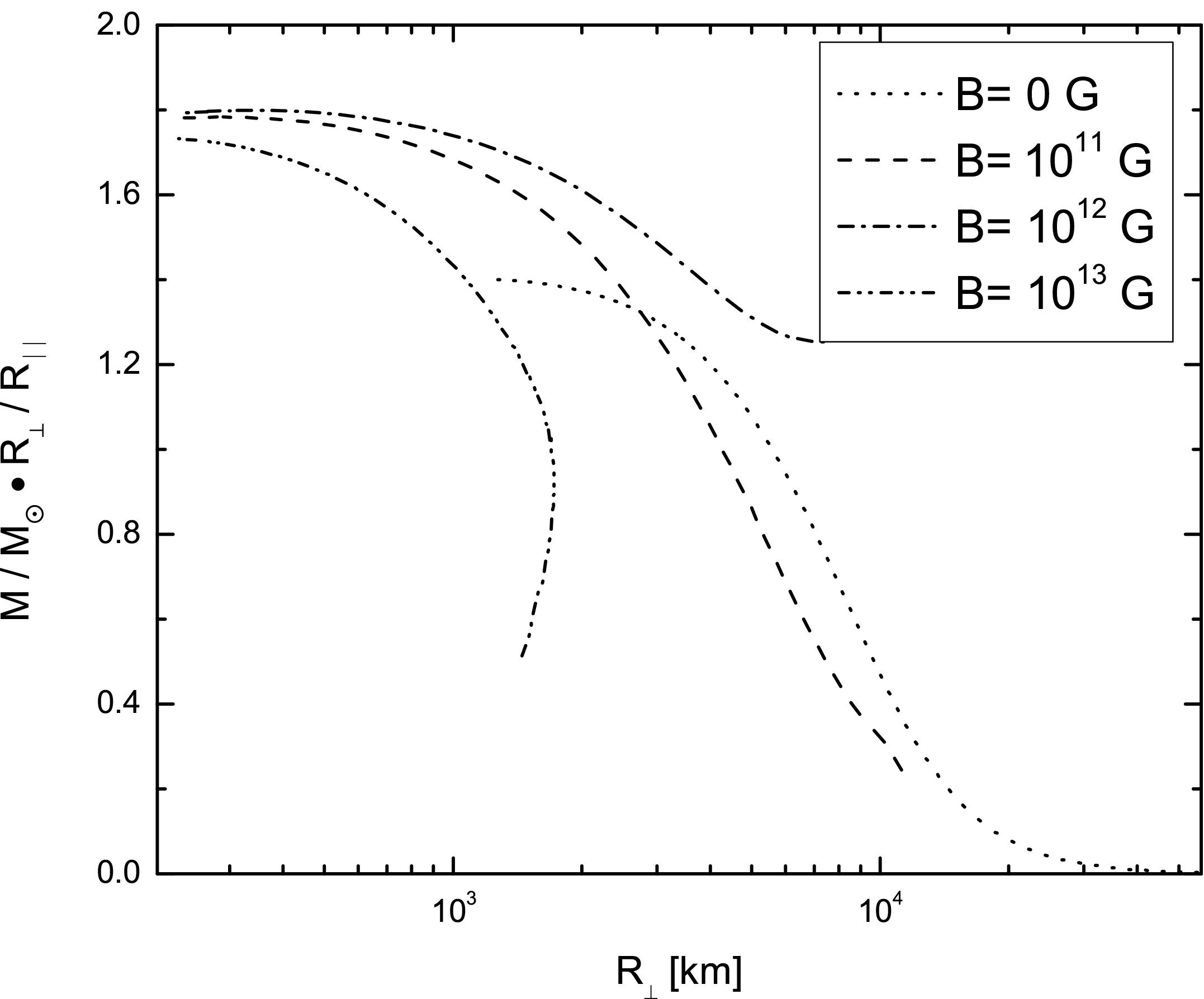
FIGURE 2 Mass-Radius relation (M R _⊥ /R _‖) in solar masses, obtained from Eqs. (16). Plots correspond to different magnetic field values: B = 0 (isotropic case R _⊥ = R _‖), B = 10¹¹ G, 10¹² G, and B = 10¹³ G. This last strength of the magnetic field is the maximum value at which stable configurations can be found. Notice that in the B 6= 0 cases, the maximum value of the magnitude (M/M _ʘ R _⊥ /R _‖) is always greater than in the isotropic case (B = 0), this does not mean that masses are greater than the Chandrasekhar limit, since the magnitude of the parallel radius is indeterminate in this model. 

Finally, Fig. 3 displays the masses and radii of the spheroidal WDs obtained with the γ structure equations, Eqs. (19), for the value B = 5 × 10¹² G and compared to the non-magnetized solution. Again, no increase in the maximum masses is found. For the chosen strength of the magnetic field, at the highest central densities and smallest radii, the mass tends to the Chandrasekhar limit (1.44 M_ʘ). However, since Eqs. (19) use both pressures (transverse and parallel) simultaneously and allow to compute the equatorial (R) and polar (Z) radii of the star, it is now possible to study the magnetic field induced deformation in a quantitatively (although approximated) way. As can be seen, from the plot, the less massive the stars, the greater their deformation, i.e. the difference between R and Z is enhanced. Also note that in the B = 0 case, the relation R = Z is fulfilled, and the curve is identical to the corresponding one in Fig. 1, as it should be, since Eqs. (19) reduce to the isotropic TOV equations.

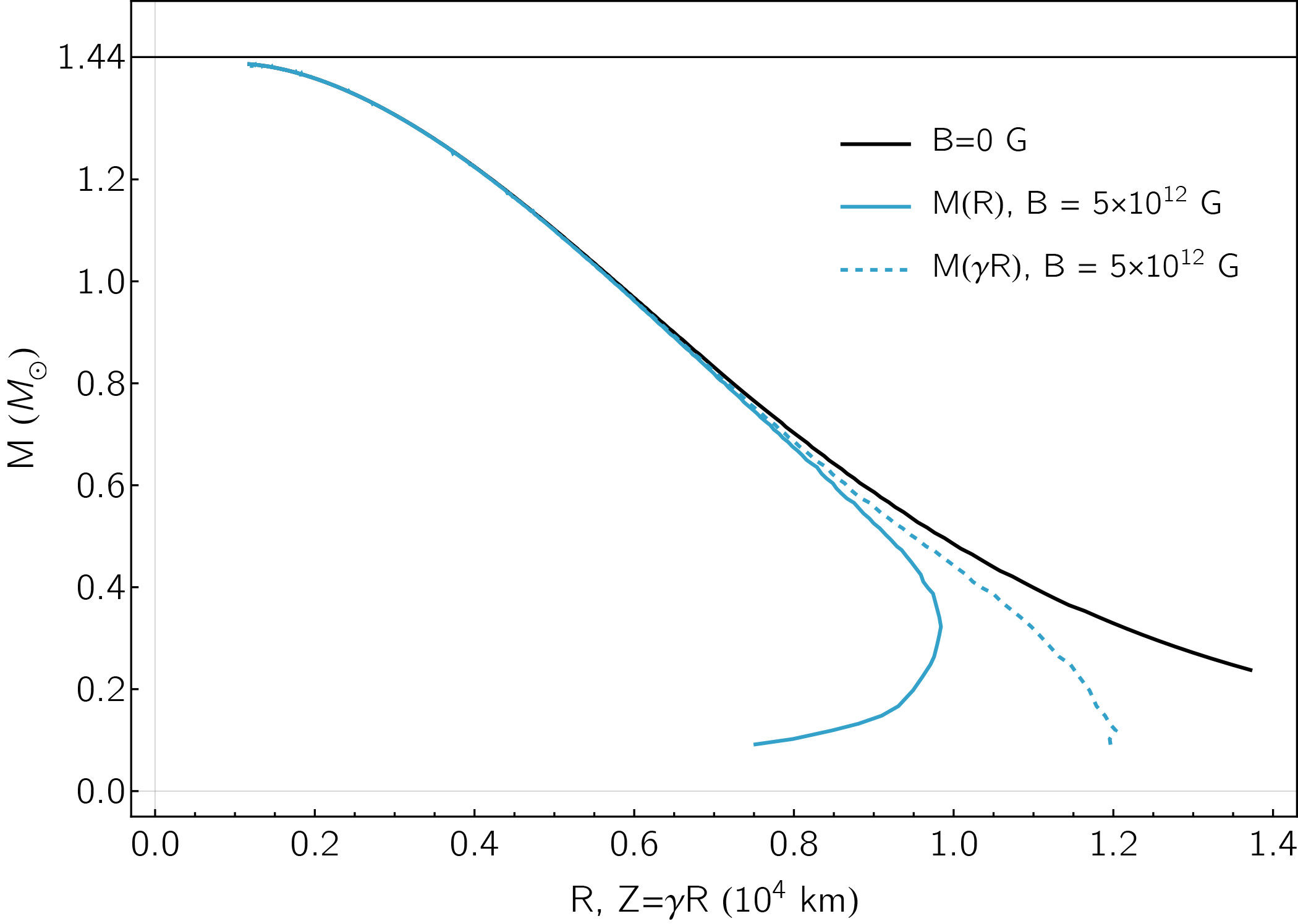
FIGURE 3 White Dwarfs mass versus the equatorial radius R and the polar radius Z obtained with the γ-structure equations Eqs. 19. 

The reviewed studies support the idea that no stable configurations for magnetized WDs are possible for super Chandrasekhar masses. On the other hand, a limiting value for the magnetic field allowed in WDs appears. It is around 10¹⁴ G, close to the critical magnetic field, B _c = 4.4 × 10¹³ G.

At this point, we should remark that, in the search for super-Chandrasekhar masses, models that assume poloidal and/or toroidal magnetic fields have been relatively successful [¹¹²]. They do find maximum masses higher than 1.4 M_ʘ; however their specific values are very model dependent. Since there is no evidence of what the shape of the field is, these results, as well as the ones presented here, are interesting but not conclusive.

5.2. Magnetized Neutron and Quark Stars

5.2.2. Magnetized Strange Quark Stars

The so-called “quark stars” (QSs) are those neutron stars composed of strange quark matter (SQM) (quarks u,d,s, plus electrons) or exotic color superconductor phases of quark matter. The simplest case is to consider a degenerate SQM star in the presence of magnetic fields, whose matter EoS are derived using Eq. (A.3), in the Appendix [¹¹⁷]. However, to have a magnetized SQM EoS compatible with the strong interaction theory, the way in which strong interactions enter in the description of matter should be defined. Many phenomenological models allow a description of the system, avoiding the complexity of QCD (where, up to now, the EoS are not well-defined).

Here, we present a work based on the phenomenological MIT Bag model, which accounts for the more important features of strong interactions: the confinement and the asymptotic freedom. In this model, quarks are considered as noninteracting particles confined to a region in space, the bag. In that case, the equations of state are [¹¹⁷]

E=∑iεi+B28π+Bbag, (21a)

P∥=∑iP∥,i-B28π-Bbag, (21b)

P⊥=∑iP⊥,i+B28π-Bbag, (21c)

where i runs over quarks u,d,s and electrons and B _bag is the vacuum energy parameter.

Equations (21) have to be complemented with stellar equilibrium conditions that guarantee charge neutrality, β equilibrium, and baryon number conservation. This is achieved by imposing the following relations

μu+μe-μd=0; μs=0,   βequilibrium, (22a)

2nu-nd-ns-3ne=0,charge neutrality, (22b)

nu+nd+ns-3nB=0, baryon number conservation. (22c)

The same study presented previously for WDs can be done in the case of magnetized Strange QS [96,118]. TOV equations are solved first for each pressure separately, then a cylindrical model is considered and, finally, the gamma structure equations are used to compute the total mass and radius. Figures 4, 5, and 6 show the mass-radius curves of magnetized QSs that result from solving TOV, the cylindrical, and the γ-structure equations with the EoS Eqs. (21), respectively. Beyond each model particularities, all the plots reflect the fact that, since the Maxwell term enters with opposite signs in both pressures, P _‖ ≤ P _⊥, a relation that is also followed by the radii associated with each pressure.

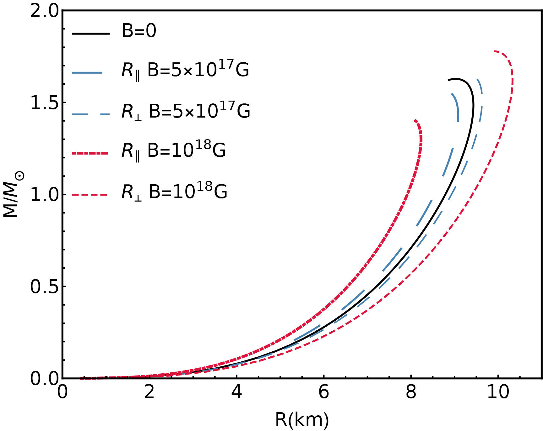
FIGURE 4 Isotropic TOV equations solutions for the perpendicular and parallel pressures independently, at B = 0 , B = 5×10¹⁷ G and B = 10¹⁸ G. 

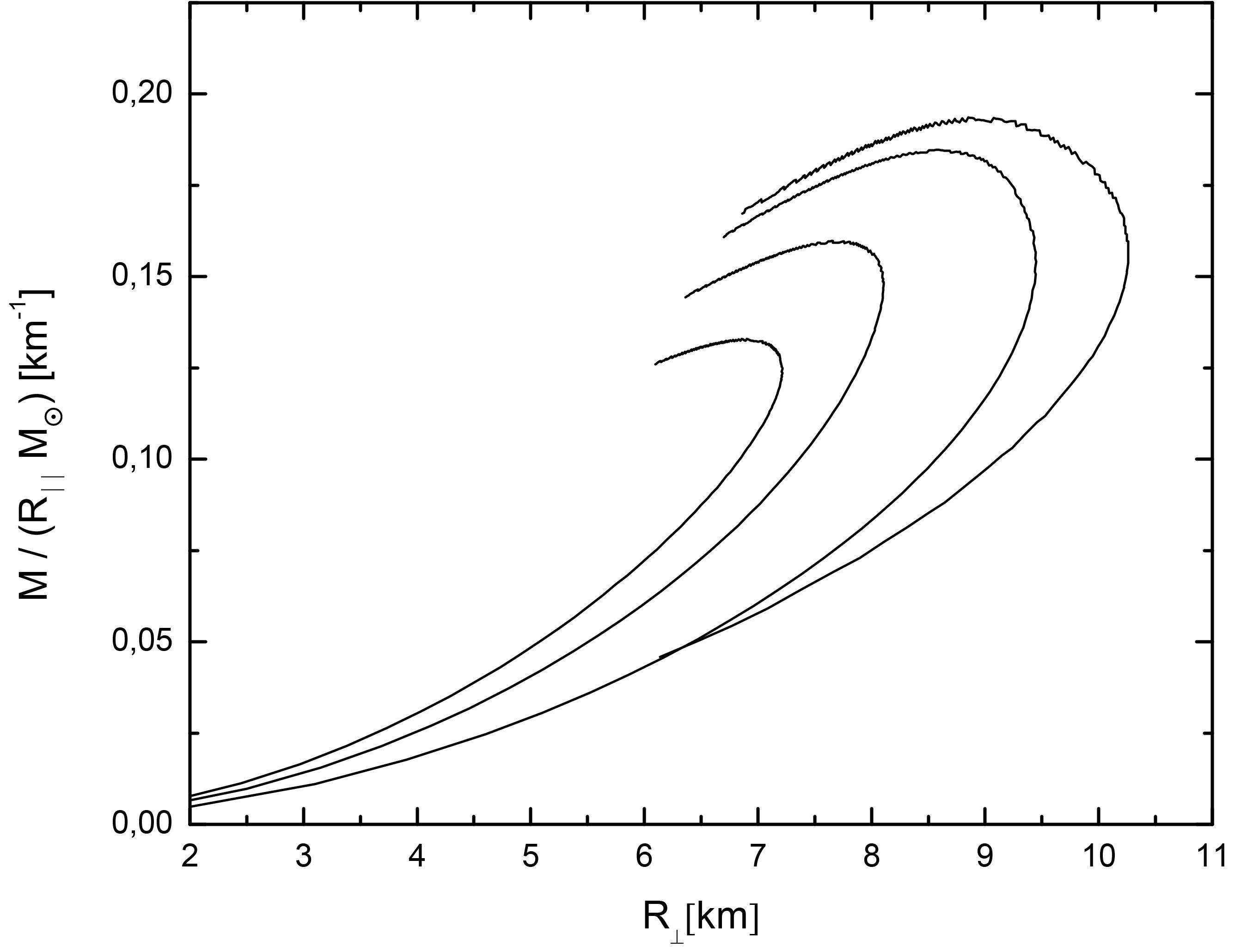
FIGURE 5 Mass per unit parallel length (M/R _k) in solar masses, vs. perpendicular radius. As the magnetic field increases, the perpendicular radius increases, up to a critical field. The curves are organized, from left to right, in order of increasing values of the magnetic field: B = 10¹⁷ G, B = 10¹⁸ G, B = 1.5×10¹⁸ G and B = 1.7×10¹⁸ G. 

FIGURE 6 Mass vs R Z, from the solutions of Eqs. (19) for magnetized quarks stars. 

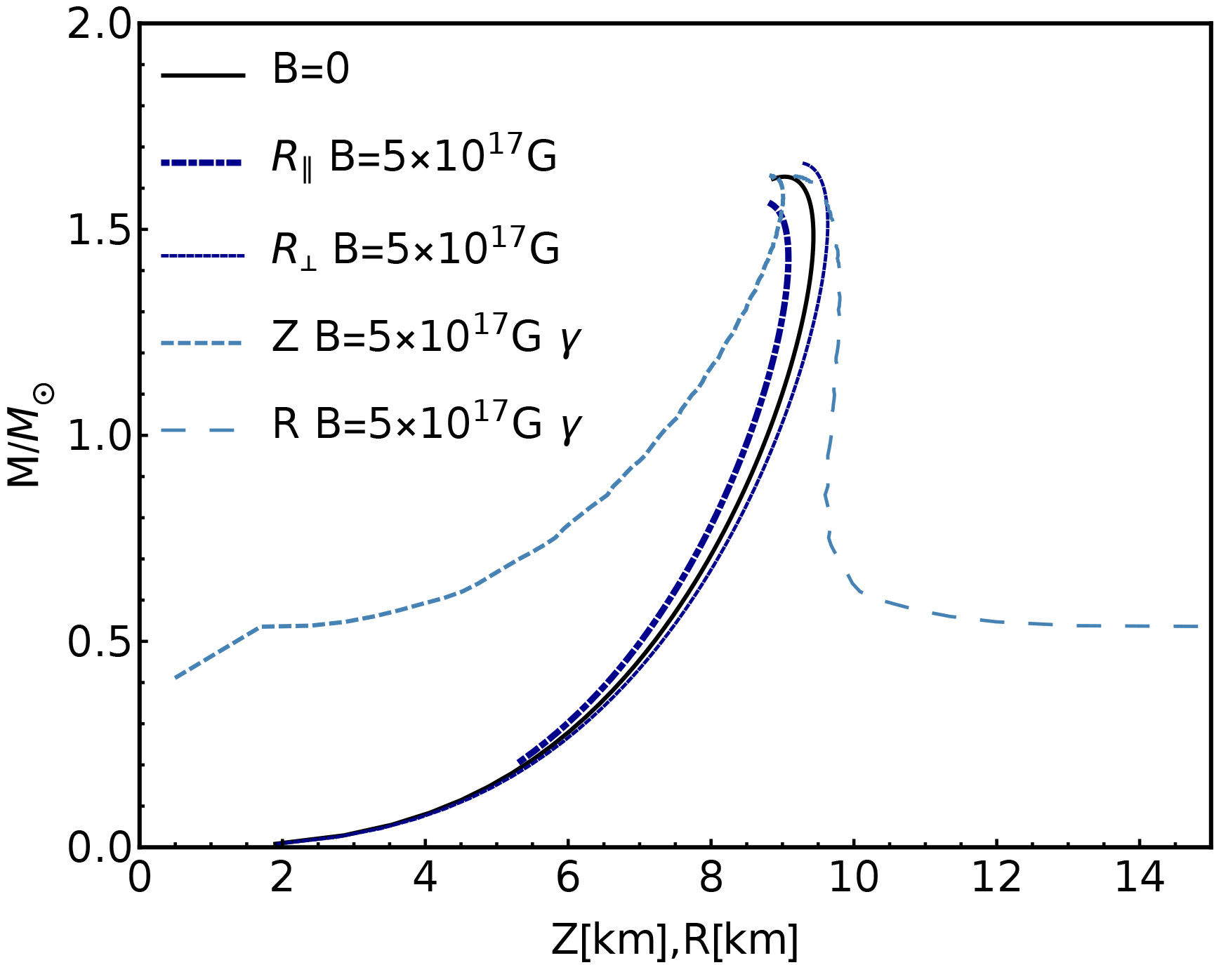
In Fig. 4, the mass-radius curves, obtained considering the pairs (Ɛ, P _‖) and (Ɛ, P _⊥) as independent EoS are presented. The non-magnetized curve is also plotted for comparison. It can be seen that, using one pressure or the other, P _‖ or P _⊥, leads to different mass-radius relations, (R _‖ ,M) and (R _⊥ ,M), respectively, whose differences increase with the magnetic field. As mentioned before, since P _‖ ≤ P _⊥ leads to R _‖ ≤ R _⊥, higher pressures give bigger stars. Also, as the mass increases, the difference in the size of the stars gets larger, suggesting that more massive stars will experience a greater deformation.

Figure 5 shows the mass (in units of M_ʘ) per unit length of a magnetized QS as a function of the equatorial radius, that results from solving Eqs. (15) with EoS Eqs. 21 [¹¹¹]. When the magnetic field increases, the perpendicular radius and the mass per unit length of the star also increase. In this work, it was found that there is a maximum field (B ∼ 1.8×10¹⁸ G) beyond which the metric coefficients exhibit a divergent behavior. This value of the magnetic field almost coincides with the threshold for which the pressure difference has become important. Therefore, the fact that no stable solutions of the system are possible beyond this point indicates the end of the theoretical stellar sequences within the adopted assumptions. Even though with this model the usual mass-radius relation cannot be computed, the information given by the model is important for constraining the maximum magnetic field allowed for magnetized strange quark stars (SQS).

The mass-radius curves given by γ-structure equations solutions for magnetized SQS, with B = 5 × 10¹⁷ G, are depicted in Fig. 6. The non-magnetized curves and the TOV solutions of Fig. 4 are also shown for comparison. The solutions show oblate objects (R > Z), as expected from TOV solutions, where R _⊥ > R _‖. Nonetheless, unlike what was found with TOV solutions, where the differences between R _⊥ and R _‖ increased with the mass, here, when Eqs. (19) are solved, the result is that the difference between R and Z decreases with the mass. The fact that the sets of structure equations, Eqs. (14) and (19), predict different qualitative behavior of the deformation induced by the presence of the magnetic field is evidence of the strong model-dependence of star observables predicted by the theoretical models [¹⁰⁶].

5.3. Magnetized BEC stars

The most common assumption about compact objects is that they are mainly composed of a degenerate fermion gas. However, a degenerate boson gas can also counterbalance gravity. Bosons at low temperatures exert almost zero thermodynamical pressure since, the lower the temperature, the greater the number of particles in the condensed state^xiv. However, even in the case of non-interacting bosons, the gravitational collapse can be stopped since, ultimately, Heisenberg uncertainty principle prevents a gas of condensed bosons to be infinitely compressed (because the relation ∆p∆x ≥ ~/2π has to be satisfied).

The first theoretical works related to stars fully composed of non-interacting bosons appeared in the sixties of the last century [¹¹⁹-¹²¹]. These models were unattractive for compact objects, since they resulted in extremely light objects whose properties could not be connected to any observed star.

Typical masses of fermion stars scale with the fermion mass m as^xv Mf ∼ (MPL3 /m2), while for boson stars the equivalent relation was Mb ∼ (MPL2 /m) [¹²⁰]. For an ideal gas of particles with m of the order of the nucleon mass, M _f ∼ 0.7 M_ʘ, while M _b ∼ 10⁻²⁰ M_ʘ However, the maximum mass of a star model can be increased by adding interactions between the particles [¹¹⁹].

A Bose-Einstein condensate star (BECS) is a star fully composed of interacting bosons formed by the pairing of two neutrons [⁷⁴,¹²²]. In a BECS, bosons counterbalance gravity thanks to the pressure that comes from their interactions. As a consequence, the strength of this interaction is what determines the maximum mass of the star, which can be as high as the nowadays desirable two solar masses [¹²²].

BECSs were proposed recently as an alternative model for NSs core [¹²²]. The main reason for their existence relies on the fact that, under certain conditions, neutron pairs formed inside NSs cores might behave as effective vector bosons. Usually, NSs cores are described as a superfluid in which nucleons couple, forming Cooper pairs. But it is well known that superfluidity is one of the limiting states of the general phenomenon of fermion pairing, being the opposite limit the Bose-Einstein condensation [¹²³-¹²⁵]. Pairing is possible for any two fermions with attractive interactions. If the pair is weakly bounded, the result is a superfluid-like behavior, while tightly bounded pairs behave as an effective boson. Due to the physical conditions inside NSs, in a more realistic model, not all nucleons have to be paired, in such a way that paired nucleons should be considered to be in an intermediate state between superfluidity and condensation. In this frame, a BECS is a limiting case in which a compact object exclusively composed of bosonized neutrons is assumed.

Considering that, in NSs cores, neutrons are expected to pair with parallel spins [⁷⁴], the effects of the magnetic field on the EoS and structure of BECS were studied in [⁷⁴]. A compact star fully composed by a gas of interacting neutral vector bosons under the action of a magnetic field, at zero temperature, is described by the EoS [⁷⁴]

where M=(κ/1-b)N, b=B/B_c being B _c = m/2κ ' 10¹⁹ G, with m and κ, twice the neutron mass and the neutron magnetic moment, respectively.

In the above system of equations, the term u ₀ N ² /2, which appears in the energy and pressures, comes from the boson-boson interaction, with u ₀ = 4πa/m. Since m is fixed, the interaction is uniquely determined by the scattering length a. The values of a are in the range of one to a few tens of fermi and, increasing them, leads to an increase in the maximum mass of the model [¹²²,¹²⁶]. The term Ω _vac (b) is the vacuum potential of a neutral vector boson gas (NVBG) [⁷⁷], and its explicit form appears in the appendix, Eq. (A.4).

Mass-radius curves of magnetized BECS are shown in Fig. 7. They were obtained by solving the γ-structure equations, Eqs. (19), with the EoS Eqs. (23), for α = 1 fm and B = 10¹⁷, 10¹⁸ G. The B = 0 curve (black curve) is also shown for reference.

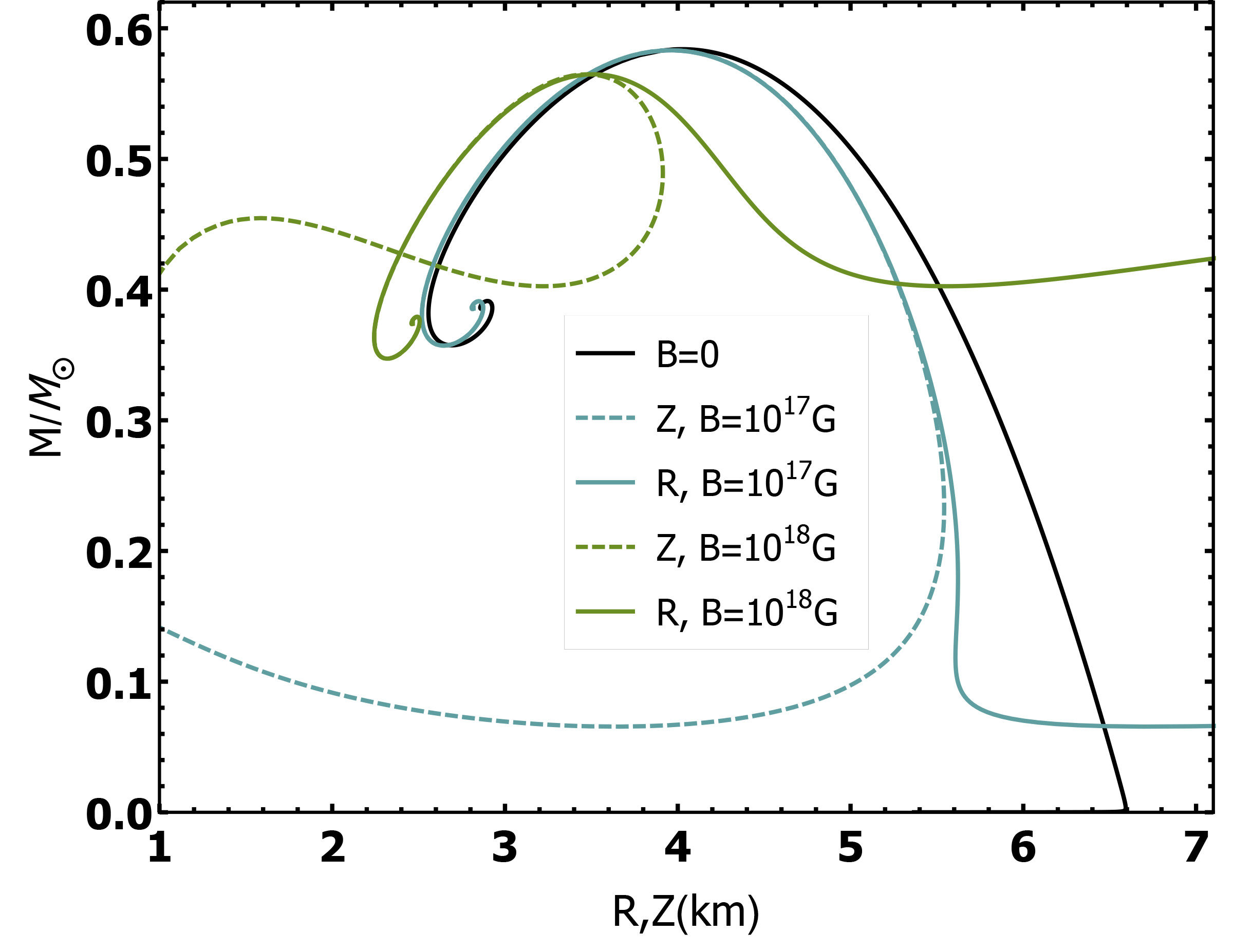
FIGURE 7 Mass-radii relations with the equatorial R (solid lines) and the polar Z (dashed lines) radius, for α = 1 fm and several values of the magnetic field. 

In contrast with the previous mass-radius plots of this paper, Fig. 7 shows the complete set of solutions of the structure equations, and not only the stable solutions (the part of the curves that are at the right of the maximum). On the other hand, let’s recall that the γ-structure equations result in spheroidal objects, in which the size of the departure from the spherical shape is determined by the magnetic field strength. As a consequence, as seen for magnetized quark stars, there are two mass-radius curves for a given value of B: the M vs Z (dashed) and the M vs R (solid) curves, corresponding to the plot of the star total mass as a function the polar (Z) and the equatorial (R) radii respectively^xvi.

As can be seen in the figure, the magnetic field presence decreases the mass and size of the stars with respect to the B = 0 case. Since Z < R, the magnetized BECS are in general oblate, although deformation is only noticeable for the less massive stars. Compared to white dwarfs and quark stars, the effects of the magnetic field are more dramatic for BEC stars. The reason for this becomes clear if we recall that bosons at T = 0 do not exert thermodynamic pressure.

5.3.1. Self-magnetization and self-generated magnetic field

In the search for the generation and preservation mechanisms of magnetic fields within COs, a candidate model that deserves some interest is the one based on spin-one bosons. A gas of spin-one bosons, below the critical temperature for condensation, exhibit a spontaneous magnetization [¹²⁷,¹³⁰]. This magnetization is not due to a spin coupling between the particles, but to the fact that bosons in the condensed phase are in the state of lowest energy. For a magnetized vector boson gas, the ground state is such that all the particles have the same spin projection (in the magnetic field direction). Consequently, spin-one gases at low temperatures generate and sustain their magnetic field [²⁴,³³,¹²⁹,¹³¹].

This self-generated field B _sg can be computed by solving the equation

Bsg=4πM, (24)

where the gas magnetization M=(κ/1-b)N, as before.

Due to the dependence of M on the particle number density, B _sg is an increasing function of the mass density ρ = mN and reaches values on the order of 10¹³-10¹⁸ G for ρ in the range of typical NS [⁷⁴,¹³¹]. On the other hand, there exists a limiting density above, which Eq. (24) does not have real solutions and the self-magnetization condition is not fulfilled. Therefore, there is an upper bound for the magnetic field that can be reached through this mechanism. For the kind of bosons considered here, the maximum mass density and magnetic field are ρ = 3.61 × 10¹⁸ g/cm³ and B = 2/3B _c , respectively. However, both the limiting density and the maximum self-generated magnetic field are far above the values expected for NS, so that the existence of a limiting density for self-magnetization is not a problem for the application of this mechanism to COs magnetic field generation.

To obtain the observables of a BECS in which the magnetic field is produced by self-magnetization, one should solve the structure equations with the EoS Eqs. (23), in which now the magnetic field intensity is not constant but given as a function of the particle density B = B _sg (ρ) by the implicit relation Eq. (24) [⁷⁴].

A significant feature that arises for B = B _sg (ρ) is that the anisotropy of the pressures is negligible [⁷⁴]. This is a direct consequence of the decrease of the magnetic field with the lessening of the mass density. Due to that, in this case, TOV equations are enough to find the macroscopic observables of the star, and the mass-radius curve does not differ substantially from that of the B = 0 case, as can be seen in the left panel of Fig. 8, for the EoS Eqs. (23), with and without considering the Maxwell terms B ² /8π.

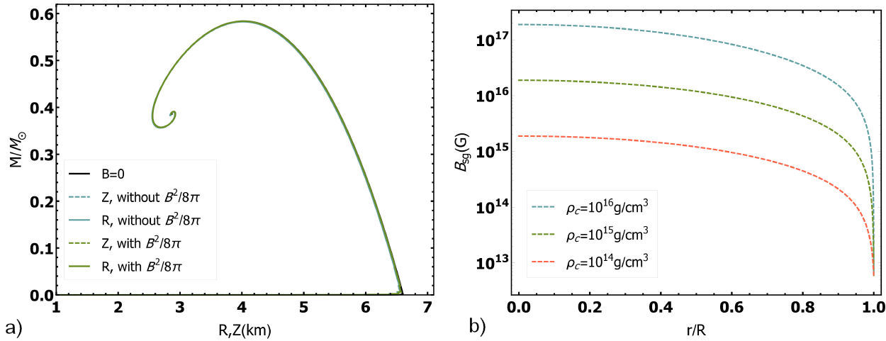
FIGURE 8 a) Mass-radius curves for BEC stars with self-generated magnetic field. b) The self-generated magnetic field in the interior of the BEC star as a function of its inner radius for several values of the central mass density of the star. 

But the most important consequence of taking B = B _sg (ρ) is that the dependence of B with the inner radius of the star may be computed while the structure equations are integrated. The magnetic field profiles for self-magnetized BECS, as a function of its radius for various central mass densities, are depicted in the right panel of Fig. 8. Note that in all cases, the values at the star center and surface are in the order of magnitude of those estimated for NS [¹¹⁴].

The profiles for the magnetic field obtained for selfmagnetized BECS validate the scenario of spin-one bosons as possible candidates for the magnetic field source, not only in that case but also for any star model whose composition includes this kind of particles. One of the merits of this scheme is that the vector boson gas can give rise to a self-generated magnetic field consistent with astronomical observations that stems naturally from the solution of the structure equations. By fixing its orientation, such a magnetic field becomes a first principle quantity free from any heuristic assumptions.

6.1. Kicks from magnetized Quarks Stars

Another phenomenon that may be influenced by the presence of a magnetic field in the interior of compact objects is the translational velocity observed for some pulsars. This velocity corresponds to a peculiar motion of a compact object with respect to the surrounding stars and to its progenitor. Data corresponding to the motion of 233 pulsars have been collected in Ref. [¹³²], where velocities as high as 1000 kms⁻¹, as well as mean velocities for young pulsar of 400 kms⁻¹, are reported. These NSs translational velocities are commonly referred to as pulsar kick velocities.

Depending on the time of their appearance, whether at birth or during the NS evolution, the kicks have been classified into natal or post-natal, respectively. Since the kick corresponds to a NS’s asymmetric motion, all the proposed models rely on some kind of asymmetric velocity producing mechanism [¹³³]. Among these we can mention the asymmetric matter ejection due to hydrodynamical perturbations during the core collapse and the supernova explosion (natal kick); the electromagnetic rocket effect produced by electromagnetic radiation along the NS spin axis from an offcentered rotating magnetic dipole (post-natal) and the asymmetric emission of neutrinos from the core of an NS in the presence of strong magnetic fields (that could be responsible for either a natal or post-natal kick, depending on the main reaction that is taking place in the core).

Several mechanisms regarding asymmetric emission of neutrinos have been proposed to explain kicks [¹³⁴,¹³⁵]. In [¹³⁶], the kick was accounted by the asymmetric emission of neutrinos due to their neutrino oscillations, relying on the fact that different neutrino species have different opacities in nuclear matter. The effect of the magnetic field is to alter the position of the resonance of the ν _τ → ν _e oscillations, depending on its orientation with respect to the neutrino momentum. In this way, τ neutrinos that escape in the direction of the magnetic field have a different temperature from those emitted in the opposite direction, carrying different momenta. In the mechanism proposed by J. Berdermann et al., [¹³⁴], the cause of the kicks is the alignment of the beaming of neutrinos along the magnetic vortex lines and the asymmetry produced by parity violation for strongly magnetized strange stars in a superconductor CFL phase. The mechanism of asymmetric emission of neutrinos coming from changing-flavor charged currents, where the polarized electron spin fixes the neutrino emission in one direction along the magnetic field, was explored in [¹³⁵].

In [¹³⁵,¹³⁶] it was shown that, when ignoring neutrino quark scattering and for typical values of temperature, density, and magnetic field strength in an NS core, it is possible to achieve kick velocities of order 1000 km/s due to asymmetric emission of neutrinos in presence of magnetic field. These large velocities receive corrections due to the smaller neutrino mean free path when neutrino interactions are included. Such interactions produce that the neutrino motion within the core quickly reaches a diffusive stage which translates into a reduced anisotropic neutrino motion. When considering these corrections, the largest kick velocities that can be obtained are of order 100 km/s, even when color superconductivity effects are included. Corrections induced from non-Fermi liquid behavior on the neutrino mean free path and emissivity beyond the leading order have also been considered in Ref. [¹³⁷,¹³⁸]. Nevertheless, other important ingredients for neutrino propagation within the core have not yet been explored (see more details in [¹³⁹]).

Following Ref. [¹³⁵,¹³⁹], a realistic scenario of asymmetric emission of neutrinos was studied, imposing stellar equilibrium conditions (β equilibrium, charge neutrality and baryon number conservation) in the core of the NS, composed by strange quark matter and taking into account the magnetic field dependence in the chemical potential and temperature of all of the thermodynamical quantities involved. The calculation is performed without resorting to analytical simplifications and for temperature, density and magnetic field values corresponding to typical conditions for the evolution of a neutron star.

In this scenario, neutrino emission comes mainly from the NS core, where the density is high enough to allow that the significant degrees of freedom are u, d, and s quarks. In this region, the emission process is driven by a flavor-changing charged current. Since in the presence of a strong magnetic field the emission is no longer isotropic due to parity violation, both neutrinos and anti-neutrinos coming from direct and inverse β decay processes, leave the NS mainly in the direction of the magnetic field, triggering an acceleration of the NS in the opposite direction. The produced kick velocity of the NS can be computed as [¹³⁵]

where M and R are the NS mass and radius, ϵ is the neutrino emissivity and χ=(Ne--Ne+/NeT) the electron spin polarization, which determines the fraction of neutrinos asymmetrically emitted. The emissivity is calculated using the cooling equation (ϵdt = −C _v dT, with C _v the heat capacity), and, through this process, the calculation of the velocity becomes a computation of an integral that involves thermos-dynamical quantities. For more details of the computation of v see [¹³⁵,¹³⁹].

In the left panel of Fig. 9, the behavior of the velocity of a typical neutron star with mass 1.4M _ʘ as a function of the neutron star radius for different values of the magnetic field and a fixed central density is shown. The right panel presents the effect on the velocity of baryon density changes: an increase in the baryon density leads to higher velocities for fixed values of the radius and the magnetic field.

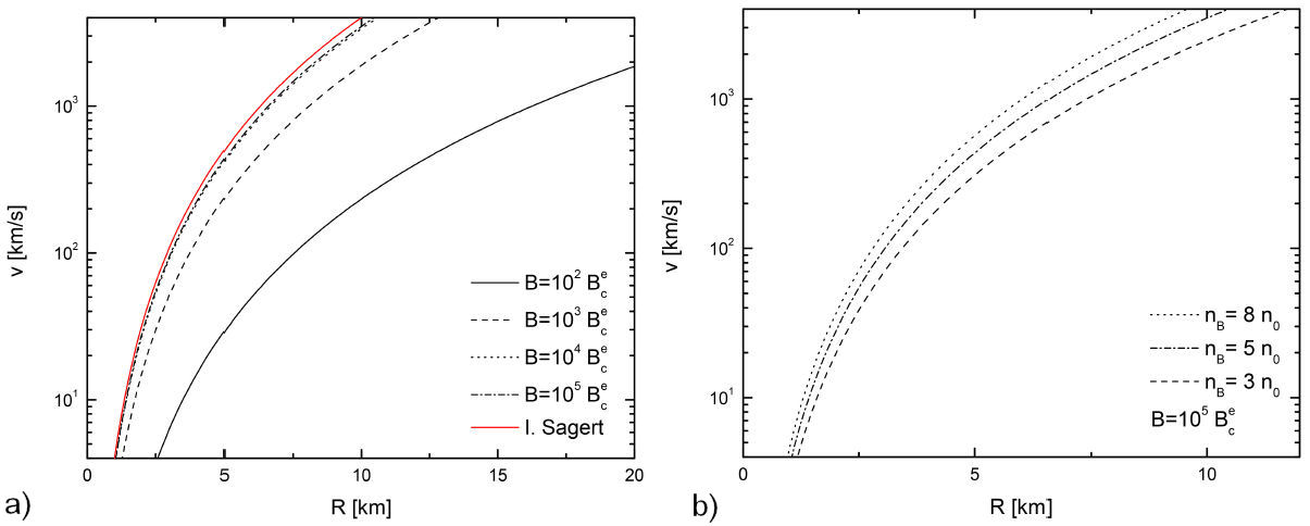
FIGURE 9 a) Kick velocity of a typical 1.4 M_¯ NS as a function of its radius, for different values of the magnetic field and a fixed central density of n _B = 5n ₀ (n ₀ = 0.16 fm⁻³) and b) for different values of the central density at a fixed magnetic field of b ≡ (B/B _cr ) = 10⁵. 

This numerical calculation, as compared with previous results, has the advantage that the inclusion of stellar equilibrium conditions and the dependence of all thermodynamical quantities on the magnetic field allows to obtain a more realistic model to describe the kick velocity mechanism and cover a wider range of magnetic field values. For instance, in Ref. [¹³⁵], some assumptions had to be made: χ = 1 (which is the strong field limit B À 10¹⁸ G), the chemical potential and temperature were fixed to 400 MeV, and 10 MeV respectively, the heat capacity was taken as independent of the magnetic field, and the stellar equilibrium conditions were not accounted for. Notice that the results shown in Fig. 9 approach those of Ref. [¹³⁶] when the magnetic field increases. The main results of this study are that, for the highest values of the magnetic field, the neutron star can reach higher velocities for smaller radii, while, for lower values of the magnetic field, the star would require a larger radius to reach velocities of the order of v _kick ∼ 1000 km s⁻¹. Summarizing, these velocities are obtained for magnetic fields that are in the range 10¹⁵ − 10¹⁸ G and radii between 20 to 5 km, respectively.

6.2. Jets from magnetized NS

It is an observational fact that, under certain conditions, stars, protostars, protoplanetary nebulae, compact objects, galaxies, and other astrophysical objects eject long streams of collimated matter that move away from their source without dispersing. Such structures are known as astrophysical jets [¹⁴⁰,¹⁴¹].

The size, velocity, and composition of jets depend on their sources. Nevertheless, their elongated form, which departs from the most common spherical or oblate shape of astronomical objects, suggests that all jets are produced and maintained by similar mechanisms. The physics behind these mechanisms is still under debate, but it is a general belief that magnetic fields play an important role in it [¹⁴⁰-¹⁴²]. In particular, two properties of magnetized quantum gases, namely, quantum magnetic collapse, and self-magnetization, seem to be crucial [⁷⁷,⁹⁵,⁹⁷,⁹⁸,¹⁴³,¹⁴⁴].

Due to the magnetic field dependent terms that appear in the spatial components of the energy-momentum tensor, the total pressures of the gas + the magnetic field system may become zero or even negative, driving the system to an instability, known as quantum magnetic collapse [¹⁴³]. In the case of gases with positive magnetization, in a regime where the magnetic pressure, −MB, dominates over the Maxwell one, B ² /8π, P _‖ > 0, while P _⊥ ≤ 0 for certain values of µ, T and B [⁷⁷,¹⁴³], so the magnetic collapse is said to be transverse. Since the effect of the negative perpendicular pressure is to push the particles inward to the magnetic field axis, the transversal magnetic collapse might be behind the onset of matter ejection and account for the jet elongated geometry. On the other hand, the magnetic field needed to keep the jet matter collimated might be produced by self-magnetization, in a way similar to the one explained above. The plausibility of such mechanisms for jet production and maintenance has been investigated recently by some of the authors of the present review [¹⁴⁵].