


 nueva página del texto (beta)
 Inglés (pdf)
 Artículo en XML
 Referencias del artículo
 Enviar artículo por email
 Citado por SciELO
  Similares en
SciELO
Similares en
SciELO 
 Permalink
1.Introduction
Hydrogen sulfide (H2S) and carbon dioxide (CO2) are called “Acid Gases” which are removed from gas streams by sweetening processes in refineries. The above are requirements either to purify a gas stream for further use in a process or environmental reasons.
The most common sweetening process is carried out by using aqueous alkanolamine solutions, which have excellent absorption characteristics and good stripping properties. Blended alkanolamines combine the absorption characteristics of the constituent amines, hence, giving higher loading capacity, faster reaction rates, and lesser energy requirement for regeneration. An example of an aqueous alkanolamines solution is the blend formed with AMP, DEA, and H2O, which has been widely studied by our researcher group 1, 2, and it is still under study in our laboratory with the aims to complete a reliable set of thermophysical and phase equilibria properties, which will define its ability to be used as a solvent for the sweetening of different hydrocarbon streams1.
Aqueous alkanolamine solutions have been used for the absorption of acid gases since 1930. The monoethanolamine (MEA) is the most alkanolamine used up to date. MEA aqueous solution is extensively used in the electric power industry for directly scrubbing CO2 from the exhaust gas produced by fossil fuel combustion 2. The physical and chemical properties of different alkanolamines, such as diethanolamine (DEA), methyl-diethanolamine (MDEA), butyl-diethanolamine (BDA), Triethanolamine (TEA), and propyl-ethanolamine (PEA), among others, have been studied by various research groups 3-6. Several studies have been published on the density of alkanolamines, due to this property plays an important role in the design, operation, and control of sweetening processes. Also, the solution density is important in the mass transfer rate modeling of absorbers and regenerators. Some studies on density are mentioned below.
Yoon et al. 2002 7 studied the density of the 2-amino-2-ethyl-1,3-propanediol + H2O mixture, which was measured by using a calibrated pycnometer at temperatures from 303.15 to 343.15 K. The density values were correlated using a quadratic polynomial equation, where predictions had an ADD of 7.05 x 10⁻² %.
The densities of aqueous blends of alkanolamines (MDEA, AMP, MEA, and DEA) at temperatures from 298.15 to 323.15 K were measured by Mandal et al. 2003 8, where a Gay-Lussac pycnometer was used. To correlate the density of liquid mixtures, a Redlich-Kister type equation for the excess molar volume was applied by Mandal et al. Their predictions show a good agreement with the experimental data, with an ADD of 0.1 %.
In 2006, Rebolledo-Libreros and Trejo 9 reported the experimental values of density for aqueous
solutions of three alkanolamines (MDEA, DEA, and AMP). The density of the
alkanolamine solutions was measured using a Sodev 03D vibrating tube densimeter. The
experimental density data were correlated by using a linear equation by
Rebolledo-Libreros and Trejo, who obtained a σ of 4 x 10⁻⁵ g
Álvarez et al. reported in 2010 10 the density of mixtures of the following alkanolamines
solutions: MEA + AMP, MEA + TEA, and MEA + MDEA, covering the entire composition
range and temperatures from 293.15 K to 323.15 K, where the experimental values of
density were used to estimate the excess molar volume. Those authors used an Anton
Paar D SA 5000 densimeter to made their experimental measurements, with uncertainty
in the density of 5 x 10⁻⁵ g
The density of the ternary solution of MDEA + MEA + ethanol (EtOH) was recently
reported by Ma et al. 2019 11, those authors used a vibrating tube densimeter to
obtain their experimental measurements in density. The excess molar volumes were
estimated from the experimental density data. The excess molar volume was correlated
by the Redlich-Kister and Cibulka’s equations. Also those authors analyzed the
intermolecular interactions of the ternary solution. Their predictions on the excess
molar volume had a σ in the range of 0.02 to 0.05 cm3
Most of the experimental works reported on phase equilibria or thermophysical properties of aqueous alkanolamine solutions have been carried out in a limited alkanolamine concentration range (e.g., between 0 to 0.2 in mole fraction 2, that corresponds to the zone rich in water), which it is commonly used in the industry.
Considering the importance of aqueous alkanolamine solutions, we carried out an experimental and theoretical study on the density of the blend formed by AMP, DEA, and H2O, covering the whole concentration range, temperatures from 303.15 to 333.15 K, and pressure of 101.3 kPa.
Two hundred sixty-four experimental points of density were measured for the ternary
mixture: AMP (1) + DEA (2) + H2O (3), with an uncertainty of 2 x
10-4 g
Besides, three prediction methods to estimate the density of the ternary mixture were tested (mixing rule, polynomial correlation, and excess molar volume), all the above methods were developed as a function of the temperature and composition of the blend, being the excess molar volume, the best method to predict the density of the ternary system studied, where the excess molar volume was correlated through the equations proposed by Redlich-Kister and Cibulka.
The importance of our work is that the experimental results on density include either pure alkanolamines or aqueous mixtures at low and high alkanolamine concentration, covering the entire concentration range. Also we develop methods to predict the density of this aqueous solution. Besides our density data can be used in the sweetening units of the refining processes, as well as in different correlations to derive other properties, like surface tension, heat capacity, and viscosity, among others. In this work, AMP, DEA, and H2O were denoted as compound (1), (2), and (3) respectively.
2.Experimental and theoretical methodology
2.1.Materials
Table I reports the characteristics of the materials that were used to carry out our study on density.
Table I Properties of the pure compounds.
| Chemical Name |
CAS |
Source |
Purification Method |
Purity |
Analysis Method |
|---|---|---|---|---|---|
| AMPa | 124-68-5 | Aldrich | Distillation | 0.995 mole fraction | GCd |
| DEAb | 111-42-2 | J.T. Baker | Distillation | 0.991 mole fraction | GCd |
| H2Oc | 7732-18-5 | - | Bidistillation | ≤ 2 × 10⁻⁶ ohm−1·cm−1 | Conductivity |
| and Deionization |
aAMP = 2-Amino-2-Methyl-1-Propanol. bDEA = Diethanolamine. cH2O = Water. dGas-liquid chromatography.
2.2.Measurements
Various blends were prepared by using an analytical balance (A&D ER-182A).
The samples were degassed using an ultrasound bath. Density measurements were
carried out in a vibrating tube densitometer (Sodev) following a methodology
reported in previous works by our research group 2, 7. Density was measured at 101.3 kPa (with an uncertainty of
0.1 kPa), and under isothermal conditions by using a Haake FK circulating bath,
where the temperature was measured using a quartz sensor joined to
Hewlett-Packard 2804A digital thermometer, with an uncertainty of 1 x
10-2 K. Density was obtained into an average period of vibration
from at least twenty stable measurements with an uncertainty of 2 x
10-4g
First, the molar volume of pure components (
where Mi is the molecular weight of the i -
th compound, expressed in g
Secondly, the molar volume of the mixture (V m ) was obtained using Eq. (2).
where x
i
is the mole fraction of the i-th compound,
Finally, the experimental excess molar volume (
2.3.Prediction methods
Three prediction methods were tested to estimate the density of pure, binary, and ternary blends formed by AMP, DEA, and H2O. The first method is based on a polynomial correlation, while the second one is based on a mixing rule; these methods were chosen due they are easy to implement as a function of temperature and concentration of the blend. The third method is based on the Redlich-Kister equation, which was chosen because it is the most frequent method to analyze the density and excess molar volume in the literature. The prediction capability of the methods used in this work was tested through four statistical parameters, which are: the relative error (ε), average absolute deviation (AAD), correlation coefficient (R), and standard deviation (σ). The mathematical expressions for each parameter are given by Eqs. (4), (5), (6), and (7).
where
where n is the number of experimental or calculated points, and AAD is the average absolute deviation expressed in %
where
where m is the number of parameters of the correlation, and σ is
the standard deviation, expressed in g
2.3.1.Polynomial correlation
We developed a polynomial correlation to estimate both the density of pure compounds and mixtures formed by AMP, DEA, and H2O.
The experimental points obtained in this work (two hundred sixty-four) were used to adjust the parameters of the polynomial correlation, where density was calculated as a function of the temperature and concentration of the blend through Eq. (8).
where
The Design-Expert v.6 software was used to adjust the parameters of the polynomial correlation, considering a two-level factorial design with three factors (x 1 , x 2 , and T). The analysis of variance (ANOVA) was made to establish the significance of the adjusted parameters.
2.3.2.Mixing rule
We used a mixing rule to predict the density of the ternary mixture. The mixing rule is given by Eq. (9), as follows:
where
While the empirical correlation for
where A, B, and C are adjustable parameters.
A FORTRAN program was codified to adjust the parameters of Eq. (10) by linear regression and using the experimental density of pure compounds.
2.3.3.Excess molar volume
This section presents the prediction methods used to estimate the excess molar volume of the binary and ternary mixtures.
2.3.3.1 Binary mixtures
The excess molar volume for the binary mixtures was correlated using the well-known Redlich-Kister equation, which is expressed as follows:
where
2.3.3.2 Ternary mixtures
The excess molar volume for the ternary mixture was estimated according to the following expression:
where
where
We considered using the methods proposed by Cibulka and Singh to estimate the ternary contribution to the excess molar volume, which are expressed as:
where B i are adjustable parameters.
3.Results and discussion
In this section, we present the main results and discussion of our study on the density of the following issues. Experimental measurements and prediction.
3.1.Pure compounds
The experimental results on density (ρ) of the pure compounds are shown in Table II. We obtained an excellent agreement with the corresponding ones that are reported in the literature; in a comparison of thirty-seven points, an AAD of 0.27% was obtained.
Table II Experimental density (ρ) of the liquid pure compounds.
| Compound | T , K | This wora | Data from literature ρg·cm−3 |
|---|---|---|---|
| 303.15 | 0.9267 | 0.9255 [2], 0.9273 [15], 0.9267 [16] | |
| AMP | 313.15 | 0.9182 | 0.9172 [2], 0.9211 [15], 0.9179 [16] |
| 323.15 | 0.9097 | 0.9092 [2], 0.9134 [15], 0.9096 [16] | |
| 333.15 | 0.9012 | 0.9007 [2], 0.9055 [1], 0.9011 [16] | |
| 303.15 | 1.0911 | 1.0909 [12], 1.09048 [17], 1.0922b [18] | |
| DEA | 313.15 | 1.0841 | 1.0847 [2], 1.0838 [12], 1.08401 [17], 1.0846b [18], 1.0843 [19] |
| 323.15 | 1.0772 | 1.0774 [2], 1.0771 [12], 1.07732 [17], 1.0781b [18], 1.0778 [19] | |
| 333.15 | 1.0702 | 1.0703 [2], 1.070 [12], 1.07174 [17], 1.0715b [18] | |
| 303.15 | 0.9953 | 0.99565 [17], 0.99565[20] | |
| H2O | 313.15 | 0.9921 | 0.99222 [17], 0.99222 [20] |
| 323.15 | 0.9882 | 0.98804 [17], 0.98804 [20] | |
| 333.15 | 0.9836 | 0.9832 [17], 0.9832 [20] |
aStandard uncertainty, ρ is 0.0002 g/cm3 and T is 0.01 K. bObtained by interpolation of values reported by DiGuillo et al.18.
3.2.Alkanolamine solutions
Table III shows the experimental results on density and excess molar volume of the blends formed with AMP, DEA, and H2O.
Table III Experimental density (ρ) and excess molar volume
(
| x1 | x2 | x3 | ρ g.cm-3 |
cm3. mol-1 |
ρ g. cm3. mol-1 |
cm3. mol-1 |
ρ g.cm3. mol-1 |
cm3. mol-1 |
ρ g.cm3. mol-1 |
cm3. mol-1 |
|---|---|---|---|---|---|---|---|---|---|---|
| 303.15 K | 313.15 K | 323.15K | 333.15 K | |||||||
| 0.9007 | 0.0993 | 0 | 0.9435 | -0.046 | 0.935 | -0.035 | 0.9265 | -0.024 | 0.9181 | -0.024 |
| 0.8006 | 0.1994 | 0 | 0.9605 | -0.097 | 0.952 | -0.076 | 0.9436 | -0.063 | 0.9352 | -0.051 |
| 0.7004 | 0.2996 | 0 | 0.9773 | -0.126 | 0.969 | -0.113 | 0.9607 | -0.097 | 0.9525 | -0.094 |
| 0.5998 | 0.4002 | 0 | 0.9942 | -0.159 | 0.986 | -0.142 | 0.9779 | -0.132 | 0.9698 | -0.126 |
| 0.5005 | 0.4995 | 0 | 1.0107 | -0.172 | 1.0026 | -0.152 | 0.9947 | -0.147 | 0.9867 | -0.137 |
| 0.3997 | 0.6003 | 0 | 1.0273 | -0.173 | 1.0193 | -0.148 | 1.0116 | -0.146 | 1.0038 | -0.14 |
| 0.3002 | 0.6998 | 0 | 1.0435 | -0.156 | 1.0357 | -0.135 | 1.0281 | -.126 | 1.0205 | -0.123 |
| 0.1998 | 0.8002 | 0 | 1.0597 | -0.127 | 1.052 | -0.099 | 1.0446 | -0.091 | 1.0372 | -0.09 |
| 0.0999 | 0.9001 | 0 | 1.0755 | -0.071 | 1.0681 | -0.053 | 1.0609 | -0.045 | 1.0537 | -0.045 |
| 0.9001 | 0 | 0.0999 | 0.9316 | -0.332 | 0.9229 | -0.309 | 0.9141 | -0.277 | 0.9056 | -0.275 |
| 0.7991 | 0.1003 | 0.1006 | 0.9512 | -0.474 | 0.942 | -0.395 | 0.9327 | -0.305 | 0.9237 | -0.243 |
| 0.6998 | 0.2001 | 0.1001 | 0.97 | -0.55 | 0.9608 | -0.463 | 0.9513 | -0.343 | 0.9418 | -0.222 |
| 0.6002 | 0.2998 | 0.1 | 0.9891 | -0.652 | 0.9797 | -0.536 | 0.9697 | -0.36 | 0.9601 | -0.22 |
| 0.4997 | 0.3996 | 0.1007 | 1.0081 | -0.734 | 0.9988 | -0.617 | 0.9885 | -0.404 | 0.9786 | -0.225 |
| 0.3997 | 0.5004 | 0.0999 | 1.0265 | -0.758 | 1.0175 | -0.656 | 1.0072 | -0.431 | 0.997 | -0.214 |
| 0.3004 | 0.5994 | 0.1002 | 1.0437 | -0.7 | 1.0352 | -0.626 | 1.0253 | -0.423 | 1.0153 | -0.212 |
| 0.1998 | 0.6992 | 0.101 | 1.0602 | -0.568 | 1.0523 | -0.528 | 1.0429 | -0.353 | 1.0336 | -0.189 |
| 0.1005 | 0.8001 | 0.0994 | 1.0757 | -0.37 | 1.0683 | -0.352 | 1.06 | -0.252 | 1.0517 | -0.158 |
| 0 | 0.8992 | 0.1008 | 1.0902 | -0.087 | 1.0835 | -0.106 | 1.0767 | -0.11 | 1.07 | -0.133 |
| 0.8004 | 0 | 0.1996 | 0.9368 | -0.604 | 0.928 | -0.57 | 0.9192 | -0.537 | 0.9105 | -0.515 |
| 0.6997 | 0.1001 | 0.2002 | 0.9583 | -0.743 | 0.9489 | -0.649 | 0.9396 | -0.562 | 0.9301 | -0.458 |
| 0.5996 | 0.2004 | 0.2 | 0.9794 | -0.842 | 0.9698 | -0.723 | 0.9597 | -0.558 | 0.9498 | -0.409 |
| 0.5002 | 0.2997 | 0.2001 | 1.0005 | -0.953 | 0.9908 | -0.816 | 0.9799 | -0.576 | 0.9696 | -0.382 |
| 0.4008 | 0.3997 | 0.1995 | 1.0213 | -1.031 | 1.0117 | -0.892 | 1.0004 | -0.61 | 0.9897 | -0.374 |
| 0.3002 | 0.4995 | 0.2003 | 1.041 | -1.013 | 1.0319 | -0.901 | 1.0208 | -0.624 | 1.0097 | -0.345 |
| 0.2001 | 0.5991 | 0.2008 | 1.059 | -0.873 | 1.0507 | -0.806 | 1.0406 | -0.594 | 1.0299 | -0.336 |
| 0.1004 | 0.6992 | 0.2004 | 1.0751 | -0.6 | 1.0677 | -0.581 | 1.0588 | -0.443 | 1.0498 | -0.302 |
| 0 | 0.8004 | 0.1996 | 1.0898 | -0.221 | 1.0832 | -0.24 | 1.0765 | -0.248 | 1.0698 | -0.265 |
| 0.6992 | 0 | 0.3008 | 0.9427 | -0.838 | 0.934 | -0.808 | 0.925 | -0.759 | 0.9163 | -0.735 |
| 0.5998 | 0.1004 | 0.2998 | 0.9657 | -0.907 | 0.9567 | -0.845 | 0.9475 | -0.768 | 0.9378 | -0.655 |
| 0.5 | 0.2001 | 0.2999 | 0.9887 | -0.983 | 0.9797 | -0.91 | 0.9695 | -0.747 | 0.9596 | -0.607 |
| 0.3997 | 0.3004 | 0.2999 | 1.0122 | -1.082 | 1.0029 | -0.977 | 0.992 | -0.752 | 0.9816 | -0.563 |
| 0.2998 | 0.4011 | 0.2991 | 1.0348 | -1.116 | 1.0257 | -1.013 | 1.0146 | -0.764 | 1.0037 | -0.527 |
| 0.1991 | 0.5007 | 0.3002 | 1.0556 | -1.026 | 1.0471 | -0.95 | 1.0367 | -0.737 | 1.0261 | -0.511 |
| 0.0999 | 0.6002 | 0.2999 | 1.0736 | -0.768 | 1.0661 | -0.741 | 1.0572 | -0.614 | 1.0478 | -0.458 |
| 0 | 0.7008 | 0.2992 | 1.0894 | -0.362 | 1.0829 | -0.38 | 1.0762 | -0.382 | 1.0695 | -0.395 |
| 0.6009 | 0 | 0.3991 | 0.949 | -1.006 | 0.9402 | -0.965 | 0.9315 | -0.935 | 0.9228 | -0.91 |
| 0.5004 | 0.0995 | 0.4001 | 0.9737 | -1.007 | 0.9654 | -0.988 | 0.9565 | -0.932 | 0.9472 | -0.853 |
| 0.3999 | 0.2007 | 0.3994 | 0.9994 | -1.053 | 0.9909 | -1.009 | 0.9813 | -0.893 | 0.9717 | -0.781 |
| 0.2995 | 0.3004 | 0.4001 | 1.0249 | -1.1 | 1.0163 | -1.036 | 1.0061 | -0.87 | 0.9959 | -0.706 |
| 0.1995 | 0.4011 | 0.3994 | 1.049 | -1.056 | 1.0408 | -1.002 | 1.0308 | -0.835 | 1.0206 | -0.659 |
| 0.0989 | 0.5001 | 0.401 | 1.0704 | -0.854 | 1.063 | -0.831 | 1.0543 | -0.727 | 1.0453 | -0.612 |
| 0 | 0.5992 | 0.4008 | 1.0887 | -0.495 | 1.0822 | -0.504 | 1.0755 | -0.501 | 1.0688 | -0.508 |
| 0.5007 | 0 | 0.4993 | 0.9562 | -1.116 | 0.9476 | -1.082 | 0.9391 | -1.06 | 0.9306 | -1.044 |
| 0.3998 | 0.0997 | 0.5005 | 0.9839 | -1.084 | 0.976 | -1.078 | 0.9675 | -1.042 | 0.9592 | -1.024 |
| 0.2998 | 0.1998 | 0.5004 | 1.012 | -1.075 | 1.004 | -1.049 | 0.995 | -0.97 | 0.9862 | -0.908 |
| 0.1994 | 0.3008 | 0.4998 | 1.0397 | -1.038 | 1.0318 | -1.002 | 1.0228 | -0.907 | 1.0135 | -0.802 |
| 0.0998 | 0.4008 | 0.4994 | 1.065 | -0.892 | 1.0577 | -0.87 | 1.0494 | -0.796 | 1.0407 | -0.709 |
| 0 | 0.4995 | 0.5005 | 1.0873 | -0.598 | 1.0808 | -0.598 | 1.0741 | -0.589 | 1.0673 | -0.586 |
| 0.3996 | 0 | 0.6004 | 0.965 | -1.184 | 0.9567 | -1.158 | 0.9482 | -1.128 | 0.9396 | -1.1 |
| 0.2994 | 0.1008 | 0.5998 | 0.9969 | -1.128 | 0.9889 | -1.102 | 0.9806 | -1.067 | 0.9728 | -1.066 |
| 0.2007 | 0.1997 | 0.5996 | 1.0275 | -1.043 | 1.0197 | -1.011 | 1.0114 | -0.96 | 1.0033 | -0.928 |
| 0.1008 | 0.2997 | 0.5995 | 1.0571 | -0.902 | 1.0498 | -0.875 | 1.042 | -0.83 | 1.0339 | -0.78 |
| 0 | 0.4006 | 0.5994 | 1.0843 | -0.648 | 1.0779 | -0.643 | 1.0713 | -0.632 | 1.0646 | -0.628 |
| 0.3008 | 0 | 0.6992 | 0.9752 | -1.178 | 0.9669 | -1.14 | 0.9584 | -1.101 | 0.9501 | -1.08 |
| 0.1987 | 0.1004 | 0.7009 | 1.01 | -0.984 | 1.0041 | -1.027 | 0.9961 | -0.992 | 0.9885 | -0.984 |
| 0.1005 | 0.2004 | 0.6991 | 1.0461 | -0.887 | 1.0388 | -0.856 | 1.0313 | -0.823 | 1.0238 | -0.801 |
| 0 | 0.3005 | 0.6995 | 1.0783 | -0.631 | 1.0721 | -0.622 | 1.0656 | -0.607 | 1.0591 | -0.604 |
| 0.1997 | 0 | 0.8003 | 0.9865 | -1.035 | 0.9787 | -0.999 | 0.9705 | -0.96 | 0.9624 | -0.933 |
| 0.0998 | 0.0995 | 0.8007 | 1.0265 | -0.77 | 1.0206 | -0.778 | 1.0133 | -0.749 | 1.0062 | -0.738 |
| 0 | 0.1998 | 0.8002 | 1.066 | 1 -0.51 | 1.0603 | -0.5 | 1.0541 | -0.485 | 1.0478 | -0.478 |
| 0.0996 | 0 | 0.9004 | 0.995 | -0.653 | 0.9885 | -0.628 | 0.981 | -0.589 | 0.9756 | -0.616 |
| 0 | 0.1002 | 0.8998 | 1.0431 | -0.302 | 1.039 | -0.316 | 1.0339 | -0.315 | 1.028 | -0.308 |
Standard uncertainties: ρ is 0.0002 g/cm3, T is 0.01 K, and x is 0.0002.
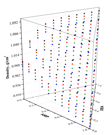
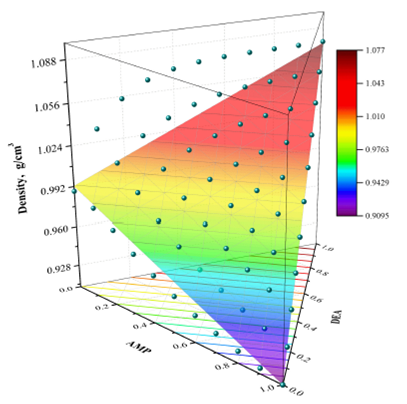
Figure 1 shows the experimental results of density in a three-dimensional (3D) plot with the shape of a triangular prism, while Fig. 2 shows projections of the experimental densities at temperatures of 303.15 to 333.15 K, where the higher values of density are located at a temperature of 303.15 K and DEA’s rich concentration zone, while the lowest values of density are located at temperature of 333.15 K, and AMP’s rich concentration zone.
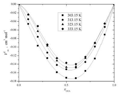
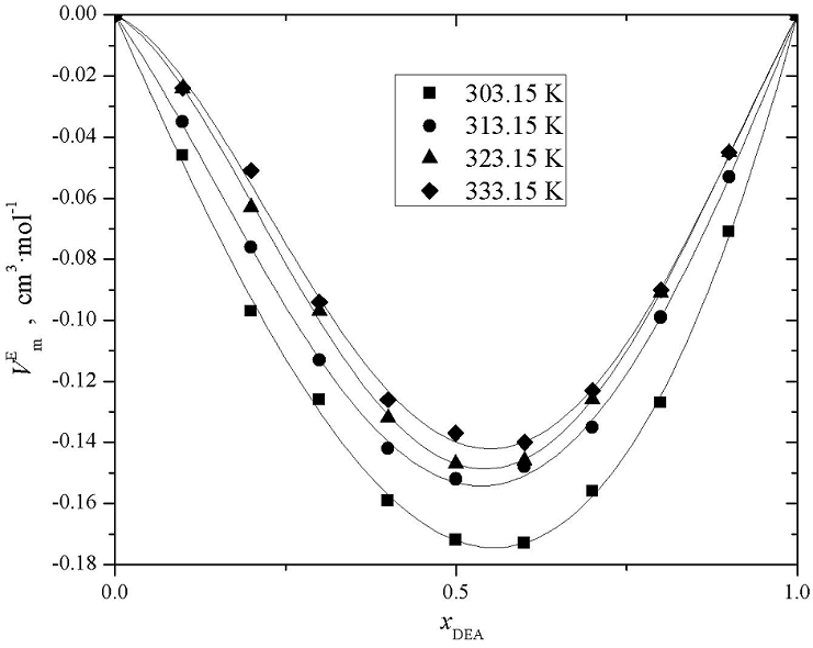
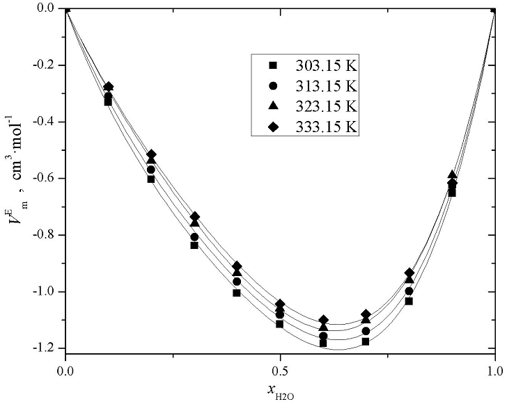
Figures 3, 4, and 5 present the
experimental excess molar volume of the binary mixtures: AMP (1) + DEA (2), AMP
(1) + H2O (3), and DEA (2) + H2O (3). Curves in plots
represent the functionality of
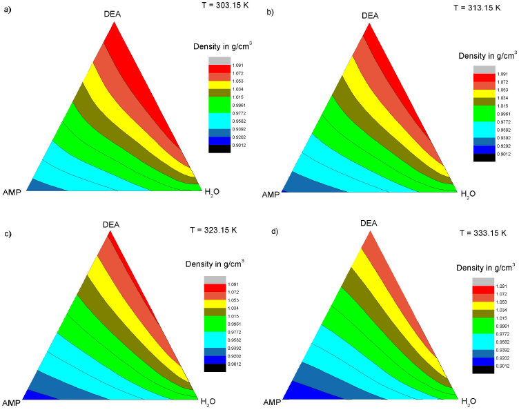
Figure 2 Projections of the experimental density data. a) 303.15 K, b) 313.15 K, c) 323.15 K, and d) 333.15 K.
3.3.Prediction methods
In this section, we present the results on the three prediction methods, as well as the statistical analysis that was carried out to test their predictive capability.
3.3.1.Polynomial test
Two hundred sixty-four experimental points were used to adjust the parameters of the polynomial correlation; the result is given by Eq. (16),
where density is a function of the temperature and concentration of the blend. We use the Gauss-Newton method to adjust the parameters of Eq. (16), through the minimization of the following objective function,
The Design-Expert v.6 software was used to minimize the objective function
using a two-level factorial design with three factors (x1,
x2, and T). The low and high levels for concentration were
fixed in 0 and 1, while the low and high levels for T were fixed in 303.15
and 333.15 K. Table IV reports the
results for the analysis of variance (ANOVA) that was obtained in this work.
Based on a 95% confidence level, the polynomial correlation was tested to be
significant, as the computed F value of 675.52 is much higher than the
theoretical F0.05 value of 2.37, which is reported for four
degrees of freedom and residual higher than 120. On the other hand, values
of “
Table IV Analysis of variance (ANOVA) for the polynomial correlation.
| Source | Sum of Squares | DF | Mean Square | F Value | Prob > F |
|---|---|---|---|---|---|
| Model based on polynomial approach | 0.6 | 3 | 0.2 | 1634.58 | < 0.0001 |
| x1 | 0.2 | 1 | 0.2 | 1616.88 | < 0.0001 |
| x2 | 0.097 | 1 | 0.097 | 789.7 | < 0.0001 |
| T | 0.023 | 1 | 0.023 | 186.8 | < 0.0001 |
| Residual | 0.032 | 260 | 1.227 × 10⁻⁴ | ||
| Total | 0.63 | 263 |
Figure 6 presents an example of the comparison between the experimental values of density and those calculated by the polynomial correlation given by Eq. (16) The experimental points are represented by points in the 3D plot, while the calculated values are represented by the colored surface, and we only show the results at 323.15 K.
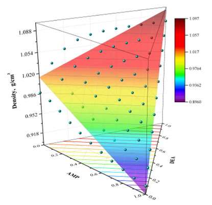
Figure 6 Experimental density data (spheres) vs. polynomial correlation (colored surface) at 323.15 K.
The statistical parameters related to the comparison between our experimental
data and the calculated values with Eq. (16) are reported in Table V. As can be seen, this method
had small values of AAD (0.82 and 1.36%) when the predictions obtained with
the polynomial correlation was compared both with our experimental data as
the data reported in the literature. However, the values of σ and R were not
satisfactory, because σ was equal to 0.0111 and 0.0162 g
3.3.2.Mixing rule test
We obtained the following equation for the mixing rule, where a dependence with temperature and concentration of the blend was incorporated:
As can be seen in Eq. (18), the density of the AMP and DEA compounds had a linear dependence with temperature, while the density of the H2O compound had a quadratic dependence. These relationships were derived by using both the experimental values of this work, as reported in the literature. Similar to the polynomial correlation, we used a linear regression to adjust the parameters of the mixing rule.
As an example, we chose the temperature of 323.15 K to show the comparison between the experimental and calculated values; the result is shown in Fig. 7, we can see that although the mixing rule offers a good approximation for most of the experimental points, there is a zone where predictions are not favorable, which is located at the rich concentration in DEA and H2O.
The results show a good agreement between experimental and calculated densities, as can be seen in Table V. With the Eq. (18) we obtained better approximations to the experimental density obtained by us than to the density reported in the literature, because in the first case, AAD and σ was smaller, and R was closer to the unit, as can be seen in Table V.
Table V Statistical parameters of the polynomial correlation and mixing rule
| Comparison | Points |
AAD % |
σ g·cm−3 |
R |
|---|---|---|---|---|
| ρcal (polynomial correlation) vs. ρexp (obtained in this work) | 264 | 0.82 | 0.0111 | 0.9745 |
| ρcal (polynomial correlation) vs. ρexp (from literature [2,5,10,14,16]) | 212 | 1.36 | 0.0162 | 0.9264 |
| ρcal (mixing rule) vs. ρexp (obtained in this work) | 264 | 1.23 | 0.0183 | 0.9676 |
| ρcal (mixing rule) vs. ρexp (from literature [2,5,10,14,16]) | 212 | 1.47 | 0.0206 | 0.9278 |
3.3.3.Redilich-Kister + Cibulka and Redlich Kister + Singh test
Table VI reports the parameters that
we obtain to predict
Table VI Parameters (A i , in cm3·mol-1) of the binary mixtures.
| AMP (1) + DEA (2) | AMP (1) + H2O (3) | DEA (2) + H2O (3) | |||||||
|---|---|---|---|---|---|---|---|---|---|
| T, K | A0 | A1 | A2 | A0 | A1 | A2 | A1 | A2 | A3 |
| 303.15 | -0.6886 | 0.1647 | 0.0238 | -4.501 | 2.1401 | -1.6665 | -2.4002 | 1.5381 | 0.3322 |
| 313.15 | -0.6126 | 0.1178 | 0.1787 | -4.3693 | 2.1341 | -1.4452 | -2.3946 | 1.4103 | 0.14 |
| 323.15 | -0.5884 | 0.1529 | 0.3131 | -4.2601 | 2.1288 | -1.0262 | -2.3589 | 1.3182 | 0.0834 |
| 333.15 | -0.5595 | 0.1752 | 0.2934 | -4.1469 | 2.1648 | -1.1516 | -2.3563 | 1.1849 | -0.0427 |
The Gauss-Newton method was used in both cases (binary and ternary systems) to adjust the best parameters able to minimize the objective function given by:
Table VIII reports the statistical parameters when the experimental excess molar volume is compared with the calculated one. The higher deviation was found at 333.15 K for the AMP (1) + DEA (2) mixture (AAD = 3.59%). The Redlich-Kister + Cibulka equations had a better performance than the Redlich-Kister + Singh et al. equations, because the first one had an AAD in the range of 1.79 to 2.18%, while the second one had an AAD in the range of 3.71 to 5.56%.
Table VIII Statistical parameters of the Redlich-Kister and Cibulka or Singh equations.
| System | Equation | T, K | Points |
AAD % |
σ cm3·mol−1 |
R |
|---|---|---|---|---|---|---|
| 303.15 | 9 | 2.1 | 0.003 | 0.9984 | ||
| AMP (1) + DEA (2) | 313.15 | 9 | 1.15 | 0.002 | 0.9993 | |
| 323.15 | 9 | 1.2 | 0.002 | 0.9995 | ||
| 333.15 | 9 | 3.59 | 0.003 | 0.9983 | ||
| 303.15 | 9 | 1.37 | 0.014 | 0.9992 | ||
| AMP (1) + H2O (3) | Redlich-Kister | 313.15 | 9 | 1.33 | 0.013 | 0.9993 |
| 323.15 | 9 | 1.15 | 0.01 | 0.9996 | ||
| 333.15 | 9 | 1.44 | 0.013 | 0.9992 | ||
| 303.15 | 9 | 0.85 | 0.005 | 0.9997 | ||
| DEA (2) + H2O (3) | 313.15 | 9 | 0.83 | 0.006 | 0.9997 | |
| 323.15 | 9 | 1.44 | 0.008 | 0.9993 | ||
| 333.15 | 9 | 1.22 | 0.008 | 0.9992 | ||
| 303.15 | 36 | 2.18 | 0.023 | 0.9937 | ||
| Cibulka 13 | 313.15 | 36 | 1.79 | 0.019 | 0.9962 | |
| 323.15 | 36 | 2.15 | 0.018 | 0.9972 | ||
| AMP (1) + DEA (2) + H2O (3) | 333.15 | 36 | 1.88 | 0.015 | 0.9986 | |
| 303.15 | 36 | 5.39 | 0.052 | 0.9736 | ||
| Singh et al. 14 | 313.15 | 36 | 5.56 | 0.049 | 0.9757 | |
| 323.15 | 36 | 5.06 | 0.035 | 0.9894 | ||
| 333.15 | 36 | 3.71 | 0.023 | 0.9969 |
After obtaining the predicted values of the excess molar volume, it is possible to re-calculate the density of the mixture using the following equation:
The above equation can be obtained from combining Eqs. (1), (2), and (3).
The excellent agreement between the experimental values and those calculated with the Redlich + Cibulka model is shown in Fig. 8. In this case, the colored surface matches very well with the experimental points at any concentration and temperature of 323.15 K. Because the Redlich + Singh model offers similar results to the Redlich + Cibulka model, the corresponding 3D plot is not included in this work.
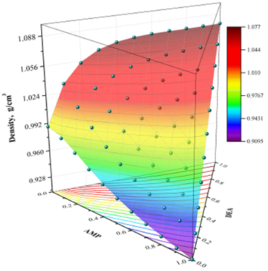
Figure 8 Experimental density data (spheres) vs. Redlich + Cibulka equation (colored surface) at 323.15 K.
The excellent agreement between the experimental and calculated values of density is also can be seen in Table IX, which shows that both prediction methods (Redlich-Kister + Cibulka and Redlich-Kister + Singh) have an excellent performance.
Table IX Statistical parameters of the Redlich-Kister + Cibulka and Redlich-Kister + Singh equations
| Comparison | Points |
AAD % |
σ g·cm−3 |
R |
|---|---|---|---|---|
| ρcal (Redlich-Kister + Cibulka) vs. ρexp (obtained in this work) | 264 | 0.02 | 0.0003 | 0.9999 |
| ρcal (Redlich-Kister + Cibulka) vs. ρexp (from literature [2,5,10,14,16]) | 212 | 0.11 | 0.0015 | 0.9995 |
| ρcal(Redlich-Kister + Singh et al.) vs. ρexp (obtained in this work) | 264 | 0.03 | 0.0005 | 0.9999 |
| ρcal(Redlich-Kister + Singh et al.) vs. ρexp (from literature [2,5,10,14,16]) | 212 | 0.12 | 0.0016 | 0.9995 |
4.Conclusions
Experimental densities were measured using the well-known vibrating tube densimeter,
obtaining reliable experimental data with an uncertainty of 0.0002 g

