On the Lagrangians and potentials of a two coupled damped Duffing oscillators system and their application on three-node motif networks

Barba-Franco, J. J.; Espinoza, P. B.; Gallegos, A.; Jaimes-Reátegui, R.; Macías-Díaz, J.E.; Barba-Franco, J. J.; Espinoza, P. B.; Gallegos, A.; Jaimes-Reátegui, R.; Macías-Díaz, J.E.

doi:10.31349/revmexfis.66.440

Servicios Personalizados

Revista

Articulo

Indicadores

Citado por SciELO
Accesos

Links relacionados

Similares en SciELO

Otros
Otros

Permalink

Revista mexicana de física

versión impresa ISSN 0035-001X

Rev. mex. fis. vol.66 no.4 México jul./ago. 2020 Epub 31-Ene-2022

https://doi.org/10.31349/revmexfis.66.440

Research

Gravitation, Mathematical Physics and Field Theory

On the Lagrangians and potentials of a two coupled damped Duffing oscillators system and their application on three-node motif networks

J. J. Barba-Franco^a

P. B. Espinoza^a

A. Gallegos^a

R. Jaimes-Reátegui^a

J.E. Macías-Díaz^b

^{^a}Departamento de Ciencias Exactas y Tecnología, Centro Universitario de los Lagos, Universidad de Guadalajara, Avenida Enrique Díaz de León No. 1144, Colonia Paseos de la Montaña, Lagos de Moreno, Jal. 47460, México. e-mail: dejesus.barba@alumnos.udg.mx; wolfgang@culagos.udg.mx; gallegos@culagos.udg.mx; rjaimes@culagos.udg.mx

^{^b}Departamento de Matemáticas y Física, Universidad Autónoma de Aguascalientes, Avenida Universidad 940, Ciudad Universitaria, Aguascalientes, Ags. 20131, México. e-mail: jemacias@correo.uaa.mx

Abstract

In this work, we investigate the Lagrangians and potentials for two coupled damped Duffing oscillators both directionally and bi-directionally. We show that, although it is not always possible to define a potential in dissipative systems, the potential of our model can be defined if the damping coefficient has a logarithmic derivative form. It is possible to apply these results to the analysis of the dynamics of complex networks based on three-node motif configurations. As an example, we study numerically the dynamics for one of the thirteen different possible configurations. Here, the phenomenon of synchronization is observed in terms of the coupling parameter.

Keywords: Duffing oscillator; motif network; Lagrangian; coupled oscillators; damped systems

PACS: 02.70.c; 03.65.Pm; 42.65.Pc

1.Introduction

The Duffing oscillator (DO) is one of the best-known nonlinear models in mathematical physics. This model was proposed by Georg Duffing to describe forced oscillations in engineering problems [¹]. However, further studies have shown that this oscillator has a wide range of applications in several contexts (see [²] and references therein). In particular, the DO has been employed in the investigation of dynamical systems and their bi-stability [³] [⁴], in bifurcation problems [⁵], in control theory [⁶] and the investigation of arrays of coupled chaotic oscillators with harmonic excitations [⁷]. Indeed, Duffing-like equations have been investigated from different points of view, especially in relation to the appearance of chaotic behavior [⁸-¹⁰]. Moreover, the study of fractional forms of those systems is an interesting open problem in nonlinear science [¹¹].

There are various works on coupled nonlinear oscillators which study their bifurcations and resonances [¹²], and the interactions between a Van der Pol oscillator and a DO [¹³]. For systems of two coupled DO’s, there are studies which focus on the bifurcation analysis for periodically driven DO’s [¹⁴, ¹⁵], chaotic synchronization [¹⁶] or on-off intermittency [¹⁷, ¹⁸]. In particular, a Lagrangian analysis is performed in [¹⁹] for two coupled undamped DO’s in order to get the corresponding integrals of motion via Noether’s theorem. However, various authors [¹⁷, ¹⁸] have noted that the damping term is very important to define a bistable system. The construction of Lagrangians for dissipative systems is nicely developed in [²⁰] but, as widely discussed in [²¹], the potential is not well defined in general for damped systems.

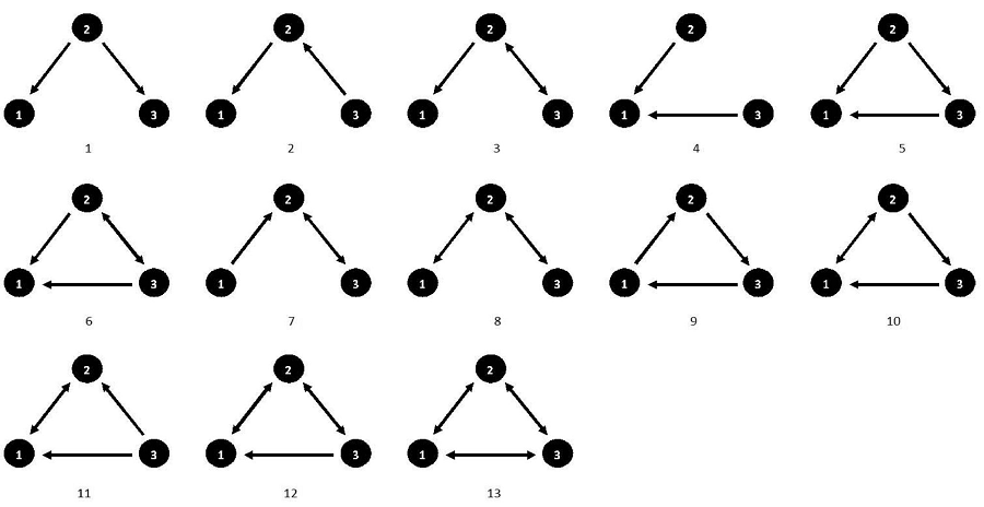
Nowadays, the study of complex networks has gathered a great relevance (see [²²] and references therein), and one can find many applications to social networks [²³, ²⁴], neural dynamics [²⁵], biology [²⁶] or chemistry [²⁷]. In [²²], a motif is defined as a pattern of interconnections occurring either in an undirected or in a directed graph at a number significantly higher than in randomized versions of the graph. The motifs play a fundamental role in complex networks. In general the motifs are defined in terms of the number of nodes. In particular, there are thirteen different configurations for a 3-node connected directed graph. The concept of motif was originally introduced in [²⁸] as the simple building block of complex networks. One can find applications of motifs, for example, in studies about chemical synthesis of topological structures [²⁹], DNA and alignment information [³⁰].

The aim of this work is to construct the Lagrangians and potentials for a two coupled damped DO’s system with directional and bi-directional interactions. The results can be used to describe the dynamics of each one of the 3-node motif network configurations. In Sec. 2, we obtain the Lagrangian for two coupled damped DO’s and show that it is not possible to get a definite potential under the presence of a constant damping coefficient. However, if the damping coefficient has the form of a logarithmic derivative then it is possible to obtain a potential function. Section 3 provides an application of the previous results on 3-node motif networks. More precisely, an illustrative example is performed following some elementary rules. In Sec. 4, we provide numerical simulations of the dynamics of the two types of damping terms discussed in this work. Finally, we close this work with a brief conclusion that summarizes the most important results of this manuscript.

2.Lagrangians and potentials

2.1.Bidirectional case

Consider two coupled identical Duffing oscillators i and j with a coupling coefficient σ. The corresponding equations of motion are

ÿi+ω02yi+δyi3+σ(yi-yj)=0,ÿj+ω02yj+δyj3+σ(yj-yi)=0, (1)

where ω02 is the squared frequency and δ is the nonlinear coefficient. Assume that σ, ω02 and δ are real numbers (though they can also be functions of the time). The Lagrangian associated to the system (1) is (see [¹⁹])

Lyij=12y˙i2+y˙j2-12ω02+σyi2+yj2-δ4yi4+yj4+σyiyj (2)

Note that if damping is to be considered in the system (1) then the resulting physical model takes on the form

ẍi+αẋi+ω02xi+δxi3+σ(xi-xj)=0,ẍj+αẋj+ω02xj+δxj3+σ(xj-xi)=0, (3)

where the damping coefficient α is a real number. In order to obtain the corresponding Lagrangian of , we may eliminate the damping term using the following transformations (see [³¹], for example):

yi=xiexp12∫αdt, yj=xjexp12∫αdt. (4)

Then the system (3) is transformed into

ÿi+-α24+ω02yi+δyi3e-αt+σ(yi-yj)=0,ÿj+-α24+ω02yj+δyj3e-αt+σ(yj-yi)=0. (5)

After comparing with the systems (1) and (2), the corresponding Lagrangian of the physical model (5) is given by

Lyij=12(ẏi2+ẏj2)-12-α24+ω02+σ(yi2+yj2)-δe-αt4(yi4+yj4)+σyiyj. (6)

Note that if (6) is written in terms of the original variables xi and xj, then the final expression of the Lagrangian is

Lxij=12x˙i2+x˙j2+α2xix˙i+xjx˙j+12α22-ω02-σxi2+xj2-δ4xi4+xj4+σxixjeαt (7)

It is easy to prove that the system (3) is retrieved from this Lagrangian employing the usual Euler-Lagrange equations.

Now, about the corresponding potential associated to the Lagrangian (7), it is well known that potentials are not necessarily defined for dissipative systems in general [²¹]. However, under certain circumstances it is possible to find a potential for the system (3). For example, in the paper [²⁰], the authors show that an oscillator of the form

ẍ+b(t)ẋ+c(x,t)=0, (8)

admits a potential of the form m(t)V(x,t) if

b(t)=ṁ/m, V(x,t)=∫xc(z,t)dz. (9)

As a consequence, the Lagrangian for (8) assumes the form

L=12m(t)ẋ2-m(t)V(x,t), (10)

where clearly m(t) can be interpreted as a variable mass. Using this result in (3) with α=α(t)=ṁ/m, the corresponding Lagrangian will have the form

Lxmij=12m(t)(ẋi2+ẋj2)-U(xi,xj,t), (11)

with a potential defined as

Uxi,xj,t=mt12ω02+σxi2+xj2+δ4xi4+xj4-σxixj. (12)

2.2.One directional case

Suppose now that the jth oscillator influences the dynamics of the ith oscillator, but not vice versa. Then the equations of this system are given by

ẍi+αẋi+ω02xi+δxi3+σ(xi-xj)=0,ẍj+αẋj+ω02xj+δxj3=0. (13)

Using the same arguments of Sec. 2.1, the Lagrangian of the ith oscillator for α constant is described by the formula

Lxi=12x˙i2+a2xix˙i+12α22-ω02-σxi2-δ4xi4+σxixjeαt (14)

Note that the coordinate xj can be viewed in this Lagrangian as a temporal function because it is a variable of another independent system. More concretely, the jth oscillator is simply an individual Duffing oscillator with Lagrangian

Lxj=12ẋj2+α2xjẋi+12α22-ω02xj2-δ4xj4eαt. (15)

When α=ṁ/m, the corresponding Lagrangians and potentials are

Lxmi=12mtẋi2-Uxi,t, (16)

Lxmj=12mtẋj2-Uxj,t, (17)

Uxi,t=mt12ω02+σxi2+δ4xi4-σxixj, (18)

Uxj,t=mt12ω02xj2+δ4xj4. (19)

3.Application on networks

In this section, we consider the 13 possible configurations for the three-node motif networks proposed in . Those configurations are shown in Fig. 1 for the sake of convenience. An emitter of the arrow is called master, while the receptor of the arrow is the slave. Of course, any node can be master and slave simultaneously, and any arrow can be bidirectional.

Figure 1 The 13 different configurations for three-node motif networks.

It is possible to describe the equations of motion, Lagrangians and potentials for each configuration using the results of Sec. 2, if we assume that the nodes are identical Duffing oscillators and follow the next rules:

If the ith oscillator is only master, then its equation is Duffing type:

ẍi+αẋi+ω02xi+δxi3=0. (20)

If the oscillators i and j are only masters, then their equations will be

ẍi+αẋi+ω02xi+δxi3=0,ẍj+αẋj+ω02xj+δxj3=0. (21)

If the ith oscillator is slave of the jth oscillator, then the equation of the ith oscillator will be given by

ẍi+αẋi+ω02xi+δxi3+σ(xi-xj)=0. (22)

If the oscillators i and j are slaves of the oscillator k, then their respective equations are

ẍi+αẋi+ω02xi+δxi3+σ(xi-xk)=0,ẍj+αẋj+ω02xj+δxj3+σ(xj-xk)=0. (23)

Finally, if the oscillator i is simultaneously slave of the oscillators j and k, then its equation will be given by

x¨i+αx¨i+ω02xi+δxi3+σxi-xj+σxi-xk=0 (24)

As an example, the equations of motion for the configuration 1 are given by the system of ordinary differential equations

ẍ1+αẋ1+ω02x1+δx13+σ(x1-x2)=0,ẍ2+αẋ2+ω02x2+δx23=0,ẍ3+αẋ3+ω02x3+δx33+σ(x3-x2)=0. (25)

Meanwhile, the Lagrangians for a constant value of α are provided by

L1=12ẋ12+α2x1ẋ1+12α22-ω02-σx12-δ4x14+σx1x2eαt,L2=12ẋ22+α2x2ẋ2+12α22-ω02x22-δ4x24eαt,L3=12ẋ32+α2x3ẋ3+12α22-ω02-σx32-δ4x34+σx3x2eαt. (26)

Finally, the Lagrangians and potentials for α=ṁ/m are

Lm1=12m(t)ẋ12-U(x1,t),Lm2=12m(t)ẋ22-U(x2,t),Lm3=12m(t)ẋ32-U(x3,t),U(x1,t)=m(t)12(ω02+σ)x12+δ4x14-σx1x2,U(x2,t)=m(t)ω022x22+δ4x24,U(x3,t)=m(t)12(ω02+σ)x32+δ4x34-σx3x2. (27)

4.Numerical results

4.1Constant damping

In this section, we analyze the behavior of the system (25) corresponding to the configuration 1 of the motif networks. To that end, we set the following values for the parameters:

α=0.4, (28)

ω02=-0.25, (29)

δ=0.5. (30)

The coupling parameter σ will be varied in order to analyze the dynamics of the system. It is important to employ adequate initial conditions. For this reason, we will use the attraction points for σ=0, which are given by

xu,d=±-ω02/δ. (31)

Here, u corresponds to the positive value and d to the negative.

Set xd as initial condition for the master oscillator x2, and xu as initial conditions for the slave oscillators x1 and x3. Clearly, the three equations are identical and independent for σ=0. Moreover, they remain constant at their initial values. However, one can see in Fig. 2 that, as σ increases, the solutions of the slaves x1 and x3 remain identical, and they tend to the attraction point of the master oscillator x2. This effect is known as synchronization in dynamical systems (see , for instance). This behavior can be explained as follows. Note that for the slave equations (x1 or x3) in , the fixed points with ẋf=0 must satisfy the condition

ω02x1+δx13+σ(x1-xd)=0. (32)

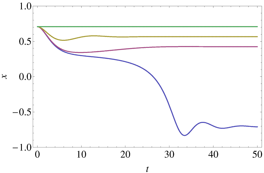
Figure 2 Solutions for the slave oscillators with α constant, for different values of the coupling parameter σ, namely σ = 0 (green), σ = 0:04 (olive green), σ = 0:06 (magenta) and σ = 0:0625 (blue).

Here, we set x2=xd because the master oscillator is fixed to this value.

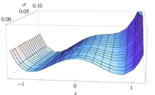
The equation (32) has three solutions:

xf=--ω02δ, xf=-ω02±-ω02-4σ2δ2. (33)

Obviously, the first solution corresponds to the attractor xd. Also, the second attractor corresponds to the second solution with positive sign, while the solution with negative sign corresponds to a repeller [³³]. Note that if

σ≥-ω02/4=0.0625, (34)

then we have only one attractor with real value xd. In other words, for these values of the coupling parameter σ, the slave oscillators will be completely synchronized with the master. For values of σ between 0 and -ω02/4, the slaves tend to the second attractor. These effects can be observed also if we integrate the left-hand side of the condition [³²] with respect to x1, and if we plot the result as a function of x1 and σ. In Fig. 3, one can readily find two wells (attractors) for 0≤σ<0.0625, and only one for bigger values.

Figure 3 Attraction wells as a function of the coupling parameter σ.

4.2.Variable damping

For this case if we propose m(t)=β(t+ϵ), where β is any realnumber and ϵ is positive and infinitesimal, then α=1/(t+ϵ). We use the same parameters and initial conditions as in Sec. 4.1 to solve the system (25). Figure 4 shows the behavior of the solutions for the slave oscillators. We used the same value of σ employed in the previous subsection, but now considering a damped oscillation. It is interesting to note that, in the present case, the potentials U(x1,t) or U(x3,t) are identical to the function graphed in Fig. 3 (up to the factor m(t)). In other words, for this second case one can use directly the defined potentials to describe the dynamics of the system.

Figure 4 Solutions for the slave oscillators with a = 1=(t + ϵ), and different values of the coupling parameter σ, namely, σ = 0 (green), σ = 0:04 (olive green), σ = 0:06 (magenta) and σ = 0:0625 (blue).

5.Conclusion

In this work, we have shown that it is possible to construct Lagrangians [³⁴, ³⁵] for two coupled damped Duffing oscillators both directionally and bi-directionally. In general it is not possible to obtain a potential for dissipative systems. However, if the damping coefficient takes the form α=ṁ/m then it is possible to define a potential. These results can be used to analyze the thirteen different configurations of the three-node motif networks. As an illustrative example, we review the dynamics for one of those configurations, using a constant damping, and a damping coefficient of the form ṁ/m. The results obtained in this work could be useful to describe the behavior of complex networks based on three-node motif configurations.

Acknowledgements

The first author wishes to thank CONACYT for the financial support granted through scholarship 924190. Also, JEMD wishes to acknowledge the financial support from CONACYT through the grant A1-S-45928.

References

1. G. Duffing, Erzwungene schwingungen bei veränderlicher eigenfrequenz und ihre technische bedeutung (Vieweg und Sohn, Brunswick, 1918). [ Links ]

2. I. Kovacic and M. J. Brennan (eds.), The Duffing Equation (John Wiley and Sons, Chichester, 2011), https://doi.org/10.1002/9780470977859. [ Links ]

3. J. S. Aldridge and A. N. Cleland, Noise-Enabled Precision Measurements of a Duffing Nanomechanical Resonator, Phys. Rev. Lett. 94 (2005) 156403, https://doi.org/10.1103/PhysRevLett.94.156403. [ Links ]

4. A. Erturk and D. J. Inman, Broadband piezoelectric power generation on high-energy orbits of the bistable Duffing oscillator with electromechanical coupling, J. Sound Vib. 330 (2011) 2339, https://doi.org/10.1016/j.jsv.2010.11.018. [ Links ]

5. U. Parlitz and W. Lauterborn, Superstructure in the bifurcation set of the Duffing equation ẍ+dẋ+x+x3=fcos(ωt), Phys. Lett. A 107 (1985) 351, https://doi.org/10.1016/0375-9601(85)90687-5. [ Links ]

6. H. Nijmeijer and H. Berghuis, On Lyapunov control of the Duffing equation, IEEE Trans. Circuits Syst. I 42 (1995) 473, https://doi.org/10.1109/81.404059. [ Links ]

7. Y. Lei and F. Guan, Disorder induced order in an array of chaotic Duffing oscillators, Int. J. Mod. Phys. C 23 (2012) 1250071, https://doi.org/10.1142/S0129183112500714. [ Links ]

8. J. Kengne, Z. N. Tabekoueng, and H. B. Fotsin, Coexistence of multiple attractors and crisis route to chaos in autonomous third order Duffing-Holmes type chaotic oscillators, Commun. Nonlinear Sci. Numer. Simul. 36 (2016) 29, https://doi.org/10.1016/j.cnsns.2015.11.009. [ Links ]

9. J. S. A. Eyebe Fouda, B. Bodo, G. M. D. Djeufa, and S. L. Sabat, Experimental chaos detection in the Duffing oscillator, Commun. Nonlinear Sci. Numer. Simul. 33 (2016) 259, https://doi.org/10.1016/j.cnsns.2015.09.011. [ Links ]

10. J. S. A. Eyebe Fouda andS. L. Sabat , A multiplierless hyperchaotic system using coupled Duffing oscillators, Commun. Nonlinear Sci. Numer. Simul. 20 (2015) 24, https://doi.org/10.1016/j.cnsns.2014.05.002. [ Links ]

11. J. Čermák, J. Horníček, and T. Kisela, Stability regions for fractional differential systems with a time delay, Commun. Nonlinear Sci. Numer. Simul. 31 (2016) 108, https://doi.org/10.1016/j.cnsns.2015.07.008. [ Links ]

12. P. Woafo, H. B. Fotsin , and J. C. Chedjou, Dynamics of Two Nonlinearly Coupled Oscillators, Phys. Scr. 57 (1998) 195, https://doi.org/10.1088/0031-8949/57/2/006. [ Links ]

13. J. C. Chedjou , H. B. Fotsin , P. Woafo , and S. Domngang, Analog simulation of the dynamics of a van der Pol oscillator coupled to a Duffing oscillator, IEEE Trans. Circuits Syst. I 48 (2001) 748, https://doi.org/10.1109/81.928157. [ Links ]

14. J. Kozlowski, U. Parlitz , andW. Lauterborn , Bifurcation analysis of two coupled periodically driven Duffing oscillators, Phys. Rev. E 51 (1995) 1861, https://doi.org/10.1103/PhysRevE.51.1861. [ Links ]

15. A. Kenfack, Bifurcation structure of two coupled periodically driven double-well Duffing oscillators, Chaos Solitons Fractals 15 (2003) 205, https://doi.org/10.1016/S0960-0779(01)00250-8. [ Links ]

16. C. Wu, T. Fang, and H. Rong, Chaos synchronization of two stochastic Duffing oscillators by feedback control, Chaos Solitons Fractals 32 (2007) 1201, https://doi.org/10.1016/j.chaos.2005.11.042. [ Links ]

17. Y. Nagai, X.-D. Hua, and Y.-C. Lai, Controlling on-off intermittent dynamics, Phys. Rev. E 54 (1996) 1190, https://doi.org/10.1103/PhysRevE.54.1190. [ Links ]

18. R. Jaimes-Reátegui and A. N. Pisarchik, Control of on-off intermittency by slow parametric modulation, Phys. Rev. E 69 (2004) 067203, https://doi.org/10.1103/PhysRevE.69.067203. [ Links ]

19. R. Naz, I. Naeem, and F. M. Mahomed, First Integrals for Two Linearly Coupled Nonlinear Duffing Oscillators, Math. Probl. Eng. 2011 (2011) 831647, https://doi.org/10.1155/2011/831647. [ Links ]

20. J. L. Cieśliński and T. Nikiciuk, A direct approach to the construction of standard and non-standard Lagrangians for dissipative-like dynamical systems with variable coefficients, J. Phys. A 43 (2010) 175205, https://doi.org/10.1088/1751-8113/43/17/175205. [ Links ]

21. R. Graham and T. Tél, Existence of a Potential for Dissipative Dynamical Systems, Phys. Rev. Lett. 52 (1984) 9, https://doi.org/10.1103/PhysRevLett.52.9. [ Links ]

22. S. Boccaletti, V. Latora, Y. Moreno, M. Chávez, and D.-U. Hwang, Complex networks: Structure and dynamics, Phys. Rep. 424 (2006) 175, https://doi.org/10.1016/j.physrep.2005.10.009. [ Links ]

23. J. Scott, Social Network Analysis, Sociology 22 (1988) 109, https://doi.org/10.1177/0038038588022001007. [ Links ]

24. M. Girvan and M. E. J. Newman, Community structure in social and biological networks, Proc. Natl. Acad. Sci. 99 (2002) 7821, https://doi.org/10.1073/pnas.122653799. [ Links ]

25. O. Sporns, D. R. Chialvo, M. Kaiser, and C. C. Hilgetag, Organization, development and function of complex brain networks, Trends Cogn. Sci. 8 (2004) 418, https://doi.org/10.1016/j.tics.2004.07.008. [ Links ]

26. A. L. Barabási and Z. N. Oltvai, Network biology: understanding the cell’s functional organization, Nat. Rev. Genet. 5 (2004) 101, https://doi.org/10.1038/nrg1272. [ Links ]

27. R. F. Ludlow and S. Otto, Systems chemistry, Chem. Soc. Rev. 37 (2008) 101, https://doi.org/10.1039/B611921M. [ Links ]

28. R. Milo et al., Network Motifs: Simple Building Blocks of Complex Networks, Science 298 (2002) 824, https://doi.org/10.1126/science.298.5594.824. [ Links ]

29. N. A. Baas and N. C. Seeman, On the chemical synthesis of new topological structures, J. Math. Chem. 50 (2012) 220, https://doi.org/10.1007/s10910-011-9907-3. [ Links ]

30. J.-J. Shu and K. Y. Yong, Identifying DNA motifs based on match and mismatch alignment information, J. Math. Chem. 51 (2013) 1720, https://doi.org/10.1007/s10910-013-0175-2. [ Links ]

31. A. Gallegos, H. Vargas-Rodríguez, and J. E. Macías-Díaz, Emakov-Lewis invariants for a class of parametric anharmonic oscillators, Rev. Mex. Fis. 63 (2017), https://rmf.smf.mx/ojs. [ Links ]

32. C. W. Wu, Synchronization in Complex Networks of Nonlinear Dynamical Systems (World Scientific, 2007), https://doi.org/10.1142/6570. [ Links ]

33. A. Fuchs, Nonlinear Dynamics in Complex Systems (Springer-Verlag, Berlin, 2013), https://doi.org/10.1007/978-3-642-33552-5. [ Links ]

34. V. Kobelev, Non-Leibniz Hamiltonian and Lagrangian formalisms for certain class of dissipative systems, Comput. Math. Meth. 1 (2019) e1035, https://doi.org/10.1002/cmm4.1035. [ Links ]

35. E. F. Combarro, J. Ranilla, I. F. Rúa, Experiments testing the commutativity of finitedimensional algebras with a quantum adiabatic algorithm, Comput. Math. Meth. 1 (2019) e1009, https://doi.org/10.1002/cmm4.1009. [ Links ]

Received: January 17, 2020; Accepted: March 23, 2020

This is an open-access article distributed under the terms of the Creative Commons Attribution License