Introduction

The study of optical soliton perturbation has been going on for several decades now [¹-⁴]. This has led to the visibility of several interesting results both from analytical and numerical perspective. While there exists an abundance of analytical tools to handle the governing equations, there exists only handful few numerical schemes that are applicable and are visible. These range from finite element method, finite difference method, Adomian decomposition scheme, Laplace-Adomian decomposition, and the variational iteration method (VIM). This paper implements VIM to address soliton dynamics, modeled by the nonlinear Schrödinger’s equation (NLSE), with a few perturbative effects. These perturbation terms come from intermodal dispersion, self-steepening effect, and nonlinear dispersion. The NLSE also includes the effect of spatio-temporal dispersion (STD) in addition to the usual chromatic dispersion (CD). The inclusion of STD, in addition to CD, makes the model well-posed. Both bright and dark solitons will be studied in the current work. The surface plot, contour plot, and the error plots are all presented for both of these solitons. The details of VIM and its application to the model are inked in the rest of the paper.

Governing model

The dimensionless form of NLSE with STD Kerr law nonlinearity is given by (5)

In Eq. (1), u(x,t) represents a complex field envelope, and x and t are spatial and temporal variables, respectively. Here, the coefficient a is the group velocity dispersion (GVD) and b is the STD the coefficient of c represents the Kerr law nonlinear term that is modeled by the functional F(|u|2)=|u|2. This type of nonlinearity originates when a light wave in an optical fiber is subjected to nonlinear responses [⁶]. Moreover, in the perturbative term of Eq. (1), the first term represents the inter-modal dispersion (IMD), the second term is the self-steepening effect and finally the last term accounts for another version of nonlinear dispersion (ND). This perturbed NLSE is going to be studied by the VIM in this paper, for Kerr law nonlinearity with fully nonlinear perturbation terms.

Solution of the perturbed NLSE ([FL-1]) equation by VIM

In this section, we outline the application of VIM to obtain explicit solution of Eq. (1) with the initial conditions u(x,0)=u0(x), ux(x,0)=u1(x). In the case of Kerr law nonlinearity where F(|u|2)=|u|2, the perturbed NLSE is given by

In the scheme of Eq. (14), we have that the linear part is R=-(αux+iauxx+ibuxt) and the nonlinear part is N=-ic|u|2u-β(|u|2u)x-γu(|u|2)x.

By applying the VIM for Eq. (21) the following recurrence relation for the determination of the components un+1(x,t); are obtained:

and so on.

Continuing in this manner, the (n+1)-th approximation of the exact solutions for the unknown functions u(x,t) can be achieved as:

Application to bright optical solitions

Consider the nonlinear Schrödinger equation with Kerr law nonlinearity (21), with initial conditions

u(x,t)=Asech[Bx]ei[-κ+θ], (27)

ux(x,0)=-ABsech[Bx]tanh[Bx]ei[-κ+θ]. (28)

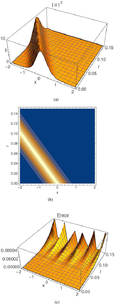
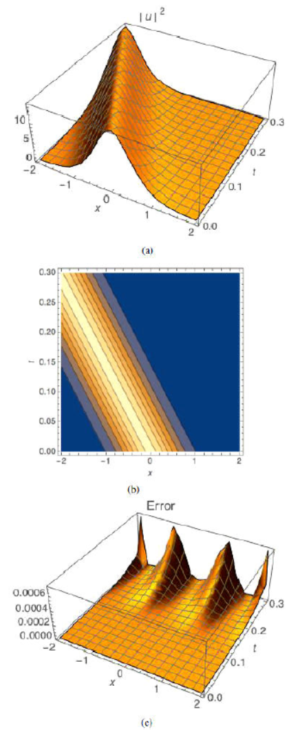
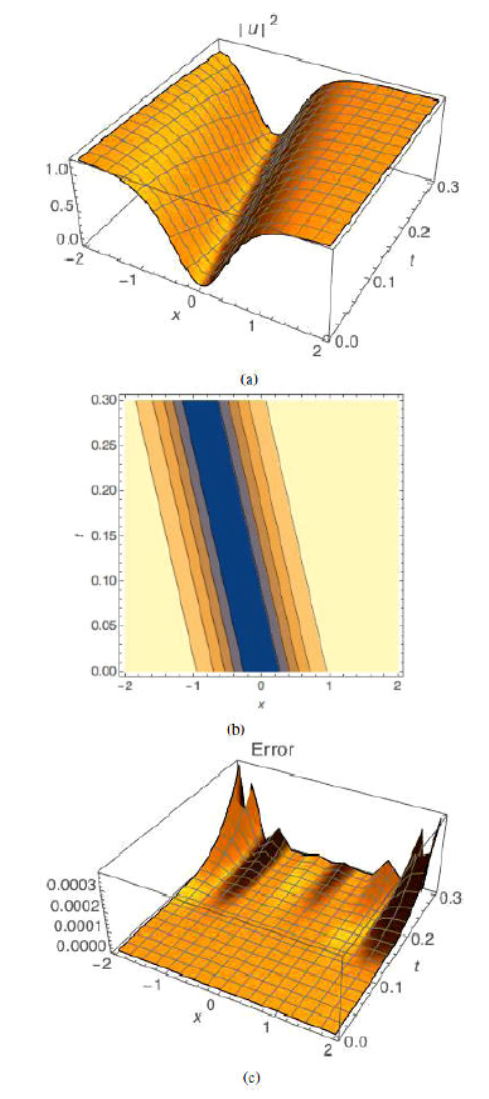
Table I shows the comparison between the absolute error of the exact and approximate solutions for various values of coefficients in the case of bright optical solitons. Figures 1, 2, and 3 give the plots for the approximate solutions by using VIM, contour plot of the wave amplitude of |u|2, and absolute error, respectively.

Table I Bright optical solitons 

Cases	a	b	c	α	β	γ	κ	ω	ν	A	B	n	|Max Error|
B1	0.1	3.2	3.8	1.5	−1.0	1.5	3.0	0.1	−29.5	3.13	2.32	14	1.5 × 10−4
B2	0.2	1.5	4.3	1.3	1.8	−2.7	1.8	−0.7	−6.93	3.81	1.63	14	6.0 × 10−4
B3	0.4	1.1	4.2	1.8	−2.1	3.1	1.3	0.5	−9.29	1.13	0.96	14	1.0 × 10−5

Figure 1 Bright solitons: Case B-1, where a) Dynamic evolution profile of |u| ² by VIM, b) Contour plot of the wave amplitude of |u| ², and c) Absolute error. 

Figure 2 Bright solitons: Case B-2, where a) Dynamic evolution profile of |u| ² by VIM, b) Contour plot of the wave amplitude of |u| ², and c) Absolute error. 

Figure 3 Bright solitons: Case B-3, where a) Dynamic evolution profile of |u| ² by VIM, b) Contour plot of the wave amplitude of |u| ², and c) Absolute error. 

Application to dark optical solitions

Consider the nonlinear Schrödinger equation with Kerr law nonlinearity ([FL-10]), with initial conditions

ux,t=A tanhBxei-κ+θ, (29)

uxx,0=-AB sech2Bxei-κ+θ. (30)

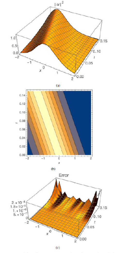
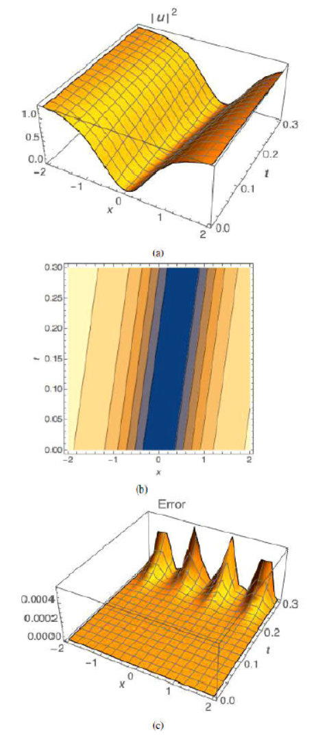
Table II shows the comparison between the absolute error of the exact and approximate solutions for various values of coefficientsin the case of dark optical solitons. Figures 4, 5, and 6 give the plots for the approximate solutions by using VIM, contour plot of the wave amplitude of |u|2, and absolute error, respectively.

Table II Dark optical solitons. 

Cases	a	b	c	α	β	γ	κ	ω	ν	A	B	n	|Max Error|
D1	2.0	1.0	3.5	1.0	−2.0	3.0	1.3	0.2	2.0	0.69	0.69	14	3.0 × 10−4
D2	2.5	1.5	4.2	1.1	−1.3	1.9	2.1	−0.1	1.8	1.12	1.20	14	4.0 × 10−4
D3	2.2	1.8	5.1	1.2	1.5	−2.2	1.2	0.3	−2.1	1.09	0.65	14	3.0 × 10−4

Figure 4 Dark solitons: Case D-1. where a)Dynamic evolution profile of |u| ² by VIM, b) Contour plot of the wave amplitude of |u| ², and c) Absolute error. 

Figure 5 Dark solitons: Case D-2, where a)Dynamic evolution profile of |u| ² by VIM, b)Contour plot of the wave amplitude of |u| ², and c) Absolute error. 

Figure 6 Dark solitons: Case D-3, where a) Dynamic evolution profile of |u| ² by VIM, b) Contour plot of the wave amplitude of |u| ², and c) Absolute error. 

Conclusions

This paper addressed the dynamics of bright and dark optical solitons governed by the perturbed NLSE that appeared with Kerr law of nonlinearity. The results are visibly meaningful with surface plots and error plots. The numerical integration scheme adopted in today’s work is VIM. Thus, the integration scheme showed a grand success with the model picked for the present study. This therefore is extremely encouraging to consider other models in future such as to study the same perturbed NLSE with non-Kerr nonlinearities and to also extend the study to optical couplers, differential group delay and with DWDM topology. Such results are in the works and will be sequentially, but surely, disseminated.

References

1. W. Yu, Q. Zhou, M. Mirzazadeh, W. Liu, and A. Biswas, Phase
shift, amplification, oscillation and attenuation of solitons in nonlinear
optics, J. Adv. Res. 15 (2019) 69,
https://doi.org/10.1016/j.jare.2018.09.001.
[ Links ]
2. A.-M. Wazwaz, A variety of optical solitons for nonlinear
Schrödinger equation with detuning term by the variational iteration method,
Optik 196 (2019) 163169,
https://doi.org/10.1016/j.ijleo.2019.163169.
3. A.-M. Wazwaz and S. A. El-Tantawy, Optical Gaussons for nonlinear
logarithmic Schrödinger equations via the variational iteration method,
Optik 180 (2019) 414,
https://doi.org/10.1016/j.ijleo.2018.11.114.
4. A.-M. Wazwaz and L. Kaur, Optical solitons and Peregrine solitons
for nonlinear Schrödinger equation by variational iteration method,
Optik 179 (2019) 804,
https://doi.org/10.1016/j.ijleo.2018.11.004.
5. M. Savescu, K. R. Khan, R. W. Kohl, L. Moraru, A. Yildirim, andA.
Biswas , Optical Soliton Perturbation with Improved Nonlinear Schrödinger’s
Equation in Nano Fibers, J. Nanoelectron. Optoelectron. 8
(2013) 208, https://doi.org/10.1166/jno.2013.1459.
6. R. Kohl, A. Biswas , D. Milovic, and E. Zerrad, Optical soliton
perturbation in a non-Kerr law media, Opt. Laser Technol. 40
(2008) 647, https://doi.org/10.1016/j.optlastec.2007.10.002.
7. J.-H. He, Variational iteration method - a kind of non-linear
analytical technique: some examples, Int. J. Non-Linear Mech.
34 (1999) 699, https://doi.org/10.1016/S0020-7462(98)00048-1.
8. J.-H. He and X.-H. Wu, Construction of solitary solution and
compacton-like solution by variational iteration method, Chaos Solitons
Fractals 29 (2006) 108,
https://doi.org/10.1016/j.chaos.2005.10.100
9. S. Momani and S. Abuasad, Application of He’s variational
iteration method to Helmholtz equation, Chaos Solitons Fractals
27 (2006) 1119, https://doi.org/10.1016/j.chaos.2005.04.113.
10. A.-M. Wazwaz , The variational iteration method for rational
solutions for KdV, / K(2,2), Burgers, and cubic Boussinesq equations, J.
Comput. Appl. Math. 207 (2007) 18,
https://doi.org/10.1016/j.cam.2006.07.010.
nueva página del texto (beta)
Inglés (pdf)
Artículo en XML
Referencias del artículo
Enviar artículo por email
Citado por SciELO