SciELO - Scientific Electronic Library Online

 
vol.66 número4Optical soliton perturbation with spatio-temporal dispersion having Kerr law nonlinearity by the variational iteration method índice de autoresíndice de materiabúsqueda de artículos
Home Pagelista alfabética de revistas  

Servicios Personalizados

Revista

Articulo

Indicadores

Links relacionados

  • No hay artículos similaresSimilares en SciELO

Compartir


Revista mexicana de física

versión impresa ISSN 0035-001X

Rev. mex. fis. vol.66 no.4 México jul./ago. 2020  Epub 31-Ene-2022

https://doi.org/10.31349/revmexfis.66.388 

Research

Atomic and Molecular Physics

Experimental setup for the production of ultracold strongly correlated fermionic superfluids of 6Li

D. Hernández-Rajkova 

J. E. Padilla-Castilloa 

M. Mendoza-Lópeza 

R. Colín-Rodrígueza  * 

A. Gutiérrez-Valdésa 

S. A. Morales-Ramíreza 

R. A. Gutiérrez-Arenasa 

C. A. Gardea-Floresa 

R. Jáuregui-Renauda 

J. A. Semana 

F. J. Poveda-Cuevasb 

G. Roatic 

aInstituto de Física, Universidad Nacional Autónoma de México, 01000 Ciudad de México, México.

bCátedras CONACyT - Instituto de Física, Universidad Nacional Autónoma de México, 01000 Ciudad de México, México.

cIstituto Nazionale di Ottica del Consiglio Nazionale delle Ricerche and European Laboratory for Nonlinear Spectroscopy (INO-CNR & LENS), 50019 Sesto Fiorentino, Italy.


Abstract

We present our experimental setup to produce ultracold strongly correlated fermionic superfluids made of a two-component spin-mixture of 6Li atoms. Employing standard cooling techniques, we achieve quantum degeneracy in a single-beam optical dipole trap. Our setup is capable of generating spin-balanced samples at temperatures as low as T/T F = 0.1 containing up to 5 x 10⁴ atomic pairs. We can access different superfluid regimes by tuning the interparticle interactions close to a broad magnetic Feshbach resonance. In particular, we are able to explore the crossover from the molecular Bose-Einstein condensate (BEC) to the Bardeen-Cooper-Schrieffer (BCS) superfluid regimes.

Keywords: Quantum degenerate gases; fermionic superfluidity; Bose-Einstein condensation; laser cooling and trapping

PACS: 67.85.-d; 67.85.Lm; 67.25.D-

1.Introduction

Quantum gases are macroscopic quantum many-body systems that represent a unique scenario to study quantum phenomena such as superfluidity and macroscopic quantum excitations [1]. Moreover, ultracold atoms have emerged as ideal quantum simulators of many-body phenomena, becoming effective testbeds of quantum Hamiltonians. Indeed, the combination of ultracold atoms and optical potentials has opened up a new way of studying condensed matter problems with unprecedented clarity [2]. This is possible thanks to the high level of controllability that quantum gases offer. The dimensionality and geometry of the system can be precisely modified by tailoring trapping potentials with laser light and magnetic fields. The thermodynamic properties of the gas, such as density, temperature, and volume can be easily manipulated. Full control of interparticle interactions is possible via magnetic Feshbach resonances [3]. Even the quantum statistics of the system can be changed by choosing fermionic or bosonic atoms. These are very powerful tools that distinguish ultracold atomic gases from ordinary condensed matter systems.

At ultralow temperatures, diluted gases composed of alkali-metal atoms interact predominantly through the s-wave scattering channel, since at such low energies, higher order collision channels are highly suppressed. In the case of ultracold bosons, Bose-Einstein condensation is possible and superfluidity emerges as long as the s-wave scattering length as has a non-vanishing value [1].

The case of ultracold identical fermions is strikingly different. In this case, s-wave scattering is also suppressed due to Pauli blocking, making these systems nearly non-interacting and, in consequence, they do not exhibit superfluid behavior even at zero temperature. The quantum degenerate state corresponds to an ideal Fermi gas, also known as Fermi sea [4].

However, it is possible to introduce interactions into the system by creating a two-component spin mixture since Pauli blocking occurs only between identical fermions, while atoms in different spin states still interact via s-wave scattering. The absolute value of as determines the interaction strength and its sign defines whether the interaction is effectively repulsive (as>0) or attractive (as<0). In fermionic systems, the interaction strength is usually described by introducing the dimensionless interaction parameter (kFas)-1, where kF is the Fermi wave vector [5]. Additionally, the existence of magnetic Feshbach resonances allows controlling the value of the scattering length practically at will by applying a constant magnetic field into the system. Therefore, varying the value of this external field makes the creation of different interaction regimes possible, from weakly to strongly interacting systems, from a repulsive to an attractive gas [3]

A very important consequence of having such control on interatomic interactions is the possibility of creating different types of bound states among the atoms. For repulsive interactions, (kFas)-1>0, a molecular bound state exists in the interaction potential. In this case, it is possible to associate diatomic molecules composed by two identical atoms which, consequently, will exhibit bosonic statistics making possible the emergence of Bose-Einstein condensation of tightly bound molecules [6-8]. On the other hand, for attractive interactions, (kFas)-1<0, the corresponding bound state occurs in momentum space due to many-body correlations at the Fermi surface, giving rise to loosely bound Cooper-like pairs whose behavior is well described by the BCS theory [9-11]. In this way, the Feshbach resonance allows to continuously transit from the BEC to the BCS regimes through the so-called BEC-BCS crossover [12-14]. The intermediate regime in which the scattering length diverges, (kFas)-1=0, known as unitary limit, is particularly intriguing because the system is strongly interacting and strongly correlated giving rise to interesting physics. Indeed, being a universal regime, physics across the BEC-BCS crossover is interesting due to its relationship with other important phenomena such as high-Tc superconductivity [15] and other strongly correlated superfluids such as neutron stars or quark-gluon plasma [16-18]. Figure 1 shows the Feshbach resonance for the case of the two lowest hyperfine Zeeman levels of 6Li, corresponding to the two Zeeman components of the absolute ground state 22S1/2 F=1/2, mF=-1/2 and mF=+1/2, which we denote as |1 and |2 respectively. Figure 1 also specifies the different superfluid states for the different interaction regimes. This Feshbach resonance is particularly broad, having a width of the order of 300G, enabling a very fine and precise control of the scattering length.

Figure 1 Feshbach resonance for the two lowest hyperfine Zeeman levels of 6Li. Different superfluid regimes are possible depending on the value of the scattering length a s

In this paper we describe our newly built setup to produce ultracold atomic gases composed by fermionic 6Li atoms in a balanced spin-mixture of the states |1 and |2. We employ a standard Zeeman slower to decelerate an atomic beam coming from an effusive oven. The decelerated atoms are trapped and further cooled down in a magneto-optical trap in which subsequently sub-Doppler cooling is used [19]. These laser cooled atoms are transferred into a single-beam optical dipole trap . Finally, quantum degeneracy is achieved by runaway evaporation. We produce ultracold samples in the different superfluid regimes across the BEC-BCS crossover containing about 5×10⁴ pairs at an approximate temperature of T/TF=0.1.

The article is divided as follows. In Sec. 2 we provide details of our experimental setup, this includes the ultra-high vacuum system, the laser system, the magnetic field generation system, and the creation of conservative potentials. Section 3 is devoted to the procedures used to cool down the gas to quantum degeneracy: laser cooling and evaporative cooling techniques, as well as details on the production of a superfluid sample in different interacting regimes. Finally, in Sec. 4, we present our conclusions and future perspectives.

2.Experimental Setup

2.1.The ultra-high vacuum system

Our ultra-high vaccum (UHV) system is divided in three main sections, namely (i) the effusive oven; (ii) the differential pumping stage, and (iii) the Zeeman slower system and the main chamber where the sample is produced and the experiments performed. Each of these sections is pumped by a 200 l/s pumping system composed by a combination of an ion pump and a non-evaporable getter (model NEXTorr D 200-5 from SAES getters Inc.). Figure 2 shows a scheme of our UHV, including a detailed cut of our main chamber.

Figure 2 Scheme of the ultra-high vacuum system including the Zeeman and the Feshbach coil systems. On the left we show a cut of the main chamber, exhibiting the distribution of the Feshbach and MOT coils. See text for details. 

The effusive oven consists of a cylindrical recipient which contains 5gr of purified 6Li. The oven is heated to a temperature of 450oC, at this temperature the vapor pressure of lithium is about 1×10⁻⁴Torr [21]. The oven is connected to the rest of the UHV system through a 4mm diameter nozzle. The vapor produced in the oven passes through this nozzle generating an atomic beam that propagates through the rest of the system. We estimate that the atomic flux of the beam effusing out from the nozzle is of the order of 6×10¹⁵atoms/s [22].

The pressure right after the nozzle reaches a value well above 10-9Torr, which is too high for producing quantum degenerate samples. To keep a sustained pressure difference between the oven and the region in which experiments are performed, we have placed a differential pumping stage which consists of two aligned tubes separated by 25mm from each other: the first one, facing the oven, has a 4.6 mm inner diameter and a second one, facing the Zeeman slower, is 7.7 mm inner diameter. This scheme is designed to keep a pressure difference across the differential pumping stage up to five orders of magnitude. In this way, the pressure in the main chamber is of the order of 10-11Torr.

The main chamber is connected to the differential pumping stage by a 56cm long and 16.5 mm inner diameter tube. Around this tube there is a conical solenoid which is used to create a spatially inhomogeneous magnetic field which is required to implement a Zeeman slower system (more details are provided in Sec. 2.3.1.).

Finally, the main chamber is a stainless steel cus- tom-made octagon chamber from Kimball Physics Inc. This chamber contains eight CF40 viewports on its sides; two CF100 vertical viewports, and ten CF16 viewports connected to the chamber by arms extruded from it at an angle of 13o from the horizontal plane. The Zeeman slower tube is connected to the main chamber by one of these arms while the Zeeman slower laser beam enters through another one diametrically opposed with respect to the center of the chamber. All viewports have anti-reflection coating for all the wavelengths used in our experiment (532nm, 671nm and 1064nm).

We have placed on both CF100 flanges reentrant viewports of high optical quality whose inner face is very close to the atoms, at a distance of only half an inch. This opens the possibility of building a large numerical aperture optical system to produce high resolution images of the sample.

2.2.Laser system

2.2.1.Optical cooling scheme

To implement the different laser cooling techniques in our experiment we use both the D2 and D1 optical transitions of 6Li [23]. We use two separate diode lasers, one for each line. The emission frequency of these lasers is locked-in into an atomic reference using a spectroscopy cell containing 5gr of purified 6Li heated at 320oC where we implement standard saturated absorption spectroscopy (SAS) [24]. We use the same cell to lock-in both lasers.

In the experiment, the D2 line is used first to implement the magneto-optical trap (MOT) and later, in the optical molasses cooling stage, while the D1 line is subsequently used to apply a sub-Doppler cooling stage. The natural linewidth of both lines is Γ=2π×5.87MHz [25]. The main optical frequencies employed in our experiment are shown in Fig. 3.

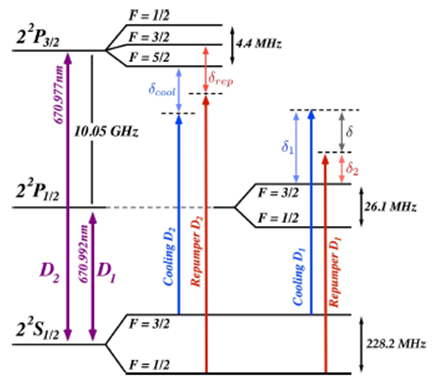
Figure 3 Level scheme (not to scale) for 6Li showing (left) the D 2 and (right) the D 1 hyperfine structures and the transitions used for the laser cooling processes. See text for details. 

To produce the D2 frequencies we have an extended-cavity diode laser (cat-eye configuration, model CEL002 from MOGLabs) which pumps an optical tapered amplifier (model MOA002 also from MOGLabs). We divide the amplified beam into two beams and independently shift the frequency of each of them using two different acousto-optic modulators (AOM). Next, each one of these beams pumps another tapered amplifier and in this way we generate two high power beams (power of 500mW each) at a wavelength of approximately 670.9 nm with a frequency difference between them of 228.2MHz, which corresponds to the hyperfine splitting of the ground state 22S1/2 of 6Li. One of these beams, the one with lower frequency, corresponds to the cooling frequency which is red-detuned from the 22S1/2(F=3/2)22P3/2 transition by 8.5Γ (about 50MHz). The second beam is used as repumper frequency and is red-detuned from the 22S1/2(F=1/2)22P3/2 transition by 8.5Γ. Note that we do not specify the hyperfine level of the excited state 22P3/2 in either the cooling nor repumper frequencies. This is because the energy levels of these hyperfine states are too close together, their separation is less than Γ, and therefore we can not resolve them in our spectroscopy cell. We superimpose both beams using a 50:50 non-polarizing beam splitter which, hence, produces two beams with the same power, each one carrying both cooling and repumper frequencies. One of these beams is used to generate the light for the MOT. To do so, we subsequently divide it into three equally powered beams and couple each one into a polarization maintaining optical fiber which brings the light directly to the experimental region. The second beam coming from this 50:50 beam splitter is additionally red-shifted by 76Γ using an additional AOM. In this way we produce the Zeeman slower beam (which also arrives into the experiment by a polarization maintaining optical fiber). This large frequency shift is chosen to match the Doppler and Zeeman shifted D2 line levels of the fast atoms coming out from the oven at the beginning of the Zeeman slower coil (where its magnetic field is maximum).

On the other hand, to implement the D1 sub-Doppler cooling stage, we require the two frequencies that are shown in the right side of Fig. 3. We have a cooling frequency blue-detuned from the transition 22S1/2(F=3/2)22P1/2(F'=3/2) by 5Γ (about 30MHz), and a repumper frequency blue-detuned from the transition 22S1/2(F=1/2)22P1/2(F'=3/2) also by 5Γ. Note that we never use both D2 and D1 lines at the same time and that the cooling and repumper frequencies of the D1 line are, evidently, also separated by 228.2MHz. This enables us to use exactly the same optical setup that we employed to generate the D2 frequencies. We have a second diode laser (same model than before) whose light we superimpose, using a polarizing beam splitter cube, onto the very same optical path of the D2 line laser. Finally, the D1 light reaches the sample using the same optical fibers that were used for the MOT. A simplified sketch of our laser setup is presented in Fig. 4.

Figure 4 Simplified scheme of the laser cooling and imaging optical setup showing the main features of the system. Lenses and waveplates have been omitted for clarity. See text for details. 

As can be seen, we essentially set all the required frequencies using three AOMs in double-pass configuration [26]. These AOMs are also used to dynamically change the frequency of these beams and implement the D2 optical molasses and D1 sub-Doppler cooling stages, as explained in Sec. 3.1.

2.2.2.Generation of probing light

The most important diagnostic tool in cold atoms experiments is imaging the samples using laser light. In our case the preferred technique is absorption imaging due to its simplicity and reliability (27),(28).

Absorption imaging consists in probing the sample using a collimated laser beam whose frequency is resonant to some atomic transition. To produce the image, we pulse this light on the atoms during a short time (of the order of 5μs). The atoms will absorb some of the light, generating an absorption profile on the beam. Finally, the light is collected by a telescope that creates an image of such absorption profile on a CCD camera (model MANTA G-145 NIR from Allied Vision Technology GmbH). The density profile of the gas can be extracted from this image [27].

In our experiment we want to produce samples at different interaction regimes across the BEC-BCS crossover. This is done by applying an external magnetic field that changes the value of the scattering length by means of a Feshbach resonance. This magnetic field, in turn, will also cause a Zeeman splitting on the electronic levels of the atoms. Hence, probing the atoms at different interaction regimes poses the necessity of generating different light frequencies to keep the imaging light resonant with the atoms.

To do so, we use the Zeeman slower beam which already has a considerable shift of -76Γ. We divert a fraction of this beam using a polarizing beam splitter before it is coupled into the Zeeman slower optical fiber, as shown in Fig. 4. Next, this diverted beam passes through additional AOMs that will further shift the frequency to match it to the specific magnetic field in which we want to probe the atoms. This configuration of AOMs allows to tune the frequency of the probing light at different values within the range from 0 to -220Γ from the D2 transitions. In this way, we are able to produce images at practically any magnetic field from 200 G to 1200 G and also at the vicinity of zero magnetic field. In this way, as can be seen in Fig. 1, we can image the sample in all the superfluid regimes across the BEC-BCS crossover, and also at weakly interacting regimes in which the gas is simply a Fermi degenerate gas but not a superfluid.

Finally, it is important to mention that the magnetic field used to access the BEC-BCS crossover is high enough to ensure that the hyperfine splitting of the atoms is well within the Paschen-Back regime, where the separation between the |1 and |2 states remains almost constant at approximately 76MHz. For this reason, we can probe both spin states in any magnetic field through the Feshbach resonance.

2.3.Magnetic field generation system

We employ three different sets of coils to generate all the required magnetic fields to trap and manipulate the atoms. We describe each of them in the following sections.

2.3.1.Zeeman slower magnetic field

We use a Zeeman slower stage to decelerate the atomic beam coming out from the effusive oven. As mentioned in the previous section, the detuning of the Zeeman slower laser beam is δZ=-76Γ for both cooling and repumper frequencies. The corresponding magnetic field along the direction of propagation of the atomic beam (direction z) is designed to decelerate atoms with velocities up to v0=960m/s at a constant deceleration akΓ/2m [29] through the formula [19]:

B(z)=μBδZ+kv02-2az, (1)

where μB is the Bohr magneton and k is the wavevector of the cooling frequency of the slower light. In this formula we only consider the cooling frequency since it is the one responsible for the deceleration of the atoms.

The mean velocity of the atoms coming out from the oven is v¯1540m/s, which is higher than the maximum velocity v0 we can decelerate in our slower. This means that, in the best case, we can only slow down about 20% of the atoms. This is not a problem since the flux of atoms effusing from the oven is very large, about 6×10¹⁵atoms/s, so we can still efficiently load our magneto-optical trap.

The magnetic field of the slower is generated by a succession of eight size-decreasing coils connected in series and an extra ninth coil at the end of the slower in which the current circulates in opposite direction, inverting in this way the direction of the magnetic field. This is known as “spin-flip configuration” [30, 31]. All nine coils are wound directly onto the slower UHV tube using 1mm diameter cooper wire. The coils are held together using a thermal conducting and electric insulating ceramic epoxy (DuralcoTM 128). The total current passing through each coil is of the order of 2.0A to generate a field which goes from a maximum around 600G to a minimum of about -250G.

Figure 5a) shows a scheme of the coil configuration of our Zeeman slower. Figure 5b) presents the generated magnetic field. Finally, Figure 5c) exhibits the calculated velocity profile of the decelerated atoms through their propagation along the slower.

Figure 5 a) Scheme of the coils of our Zeeman slower, the number of windings of each coil is indicated in the format H x V , where V denotes the number of layers in the vertical direction and H provides the number of turns in each layer. b) Axial component of the magnetic field generated along the Zeeman slower, the blue dots are the experimental data, the orange dashed line is the simulated field for this coil configuration and the solid green curve is the ideal magnetic field obtained through Eq. (1). The data uncertainty is of 1% however the corresponding error bars are not visible at this scale. c) Evolution of the speed of the atoms propagating through the Zeeman slower, the dashed horizontal line indicates the capture velocity of the MOT. 

2.3.2.Magnetic quadrupole

To produce the magneto-optical trap we use a quadrupole magnetic field whose axial gradient at the center of the trap is Bz(z)/z|z=028G/cm. This field is generated by two small coils of 6×4 windings connected in anti-Helmholtz configuration. Each of these coils is mounted in a cylindrical water-cooled support to prevent them from heating. This support is made of TeflonTM, which is a non-magnetic and insulating material, this prevents eddy currents from being induced in it when the quadrupole field is abruptly varied. Both supports are mounted inside the reentrant viewports of the main chamber, along the vertical direction. The coils are wound with strip-shaped copper wire of 4mm × 1mm and held together with ceramic epoxy (DuralcoTM 128). Figure 2 shows the position of these coils in the main chamber.

2.3.3.Feshbach resonance magnetic field

As already mentioned, one of the important advantages of ultracold lithium gases is the possibility of controlling interatomic interactions with a high degree of precision by means of a Feshbach resonance [3]. [6]Li presents several Feshbach resonances whose characteristics depend on the internal state of the interacting atomic pair. We will use the resonance between states |1 and |2, shown in Figure 1, centered at 832G. So we need an extra set of coils that are able to produce an uniform magnetic field with any value from zero to 1000G in order to have full control of all interaction regimes. To do so we have a pair of coils connected nearly at Helmholtz configuration. We deliberately move slightly away from the Helmholtz configuration so the magnetic field presents a small curvature, which will be useful to confine the atoms along the weak direction of our optical dipole trap; right at the Feshbach resonance, at 832G, this curvature along the coils axis direction is Bz(0)=6.2G/cm2, while the corresponding magnetic gradient is nearly zero (see Sec. 2.4 for more details).

The Feshbach coils are made by 4mm square section copper wire. This wire is hollow, with an internal diameter of 2mm, which allows cooling the coil by circulating cold water inside the wire. These coils were fabricated by the company Oswald Elektromotoren GmbH and each of them is embedded in an insulating resin that avoids the induction of undesired eddy currents. We can circulate a current above 200 A without noticing any significant heating of the coils. This thermal stability together with a PID feedback loop makes possible to produce magnetic fields with a stability of one part in 104. We place these coils along the vertical direction, colinear to the quadrupole field coils. Figure 2 shows each of the employed set of coils and their position in the experimental setup.

2.4.Conservative trapping potential

We produce the quantum degenerate fermionic system in a conservative trap generated by the combination of an optical potential and a magnetic curvature.

The optical potential consists in a far red-detuned single-beam optical dipole trap (ODT) created by focusing a gaussian infrared laser beam [20]. We use a single mode ytterbium-doped fiber laser from IPG Photonics Corp. (model YLR-200-LP) which delivers up to 200W of continuum linearly polarized infrared light at λ=1070nm. The beam of this laser is coupled into an acousto-optic modulator and the first diffracted order is used to produce the optical trap. We use a quartz crystal AOM that withstands very high intensities, above 1GW/cm2, from the company Gooch & Housego (model I-M080-2C10G-4-AM3). The diffraction efficiency of this AOM and, consequently, the power of the ODT, is manipulated by controlling the amplitude of the RF signal that drives the modulator using an external analog signal. To stabilize the power of this diffracted order, we employ a PID circuit driven by the signal of a photodiode (Thorlabs, model DET36A) that detects the small fraction of the light of this beam that is transmitted by a 99.9% reflection mirror.

Next, we collimate the beam at a diameter of approximately D=5.5mm and finally use a f=40cm focal length lens to focus the light on the atoms. The beam waist at focus is w0=2λf/πD50μm, which corresponds to a Rayleigh length of zR=πw02/λ=7.34mm.

The trap frequencies of this single beam ODT along the radial and axial directions are given, respectively, by [20]

ωrODT=4U0mw02andωzODT=2U0mzR2, (2)

where U0 is the depth of the trapping potential and it is given by [20]

U0=3πc2Γ2ω03ΔωI0, (3)

where ω0 is the frequency of the lowest energy optical dipole transition of the 6Li atom, which corresponds to the D1 transition, Γ is the natural linewidth of such transition and Δω=ω0-ω is the detuning between such transition and the ODT laser frequency ω. Finally, I0 is the intensity of the ODT beam at focus, I0=2P/πw02, where P is the power of the ODT laser.

This trap provides a tight confinement along the radial direction of the beam, however, along the axial (or propagation) direction it is very weak. For instance, at the end of the evaporative cooling where the power of the ODT laser is approximately P=35 mW (see Sec. 3.2.2), the radial and axial frequencies of the optical trap respectively are ωr=2π×163Hz and ωz=2π×0.94Hz, which would provide an extremely elongated sample with an aspect ratio larger than 1:160.

For this reason, we add to the optical potential a magnetic curvature that provides a better confinement along the axial direction. As mentioned in Sec. 2.3.3, we produce such curvature by setting the Feshbach coils slightly off the Helmholtz configuration. In this way, we create a saddle-point magnetic potential of the form [28, 32]

Umag(r,z)=m2ωzmag2z2-ωrmag2r2, (4)

where the trap frequencies are determined by the curvature of the field component along the corresponding direction, i.e. ωzmag2=μBz(0)/m and ωrmag2=μBr(0)/m, being m the mass of 6Li atom and μ the magnetic moment of the trapped state which, in general for the ground state of alkali atoms, is of the order of the Bohr magneton, μμB.

Note from Eq. (4) that along the radial direction we have an “anti-curvature” which will tend to deconfine the atoms along that direction. The total frequencies of our hybrid trap will be given simply by

ωr=ωrODT2-ωrmag2andωz=ωzODT2+ωzmag2. (5)

In our experiment, once the quantum sample is produced, we have that the radial optical confinement is much larger than the magnetic one (ωrωrODT), and, vice versa, along the axial direction the confinement is dominated by the magnetic component (ωzωzmag).

The axial curvature generated for the fields used to access the BEC-BCS crossover is of the order of Bz(0)=6.2G/cm2 which, superimposed to the ODT potential, translates into a total axial frequency of ωz2π×11Hz. In this way we obtain a cigar-shaped quantum sample whose aspect ratio, of the order of 1:15, is appropriate for our goals.

3.Methods and results

In the following sections we provide details on the experimental procedures employed to produce the ultracold samples.

In a very general way, the production of the quantum sample can be divided into two main processes: (i) an initial laser cooling stage mediated by absorption and reemission of light, explained in Sec. 3.1, and (ii) transference into a conservative potential and cooling by forced evaporation, presented in Sec. 3.2

3.1.Implementation of laser cooling technique

In this first cooling process we are able to produce atomic samples at temperatures as low as 40 μK containing 4.5×10⁸ atoms with a density of the order of 4.5×10⁹ atoms/cm3, which correspond to a phase-space density of about 6.6×10⁻⁶. We provide details on the laser cooling procedure in the following sections.

3.1.1.Zeeman slower and magneto-optical trapping

Zeeman slower operation

The quantum sample generation process starts by heating the lithium sample contained in the oven of our UHV system to 450oC . This generates a high temperature atomic beam that propagates through the UHV system towards the main chamber. The atoms of this beam undergo a first cooling process as they are decelerated by our Zeeman slower. Along the slower, a laser beam propagates in the opposite direction to the atomic beam. This laser carries two different frequencies, both of them red-detuned by 76Γ (446 MHz) from the cooling and repumper transitions of the D2 line. Each of these frequencies has a power of 40mW and carries positive circular polarization σ+. In this way, we are able to decelerate all the atoms from velocities classes under 960m/s to speeds of the order of 40m/s, well below the 60m/s capture velocity of the MOT, as shown in Fig. 5c).

We found that controlling independently the electric current of the spin-flip coil provides better results. Best results are obtained using a current of 2.0A for the spin-flip coil and 2.9A for all other coils, which optimize the number of loaded atoms into the MOT and minimize the corresponding loading time.

Loading of the magneto-optical trap: The decelerated atoms arrive into the main chamber where we capture them and further cool them in a magneto-optical trap (MOT) [19]. To implement the MOT we use three retroreflected mutually perpendicular laser beams with a diameter of D=2.3cm, as shown in Fig. 6.

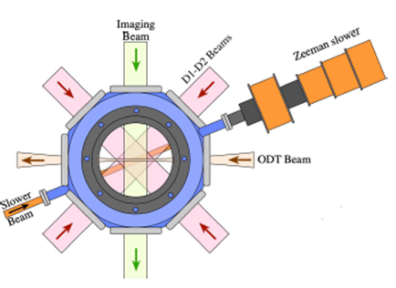
Figure 6 Top view scheme of the main chamber, showing the configuration of the MOT beams (D1 and D2 beams), the imaging beam, the Zeeman slower beam and the ODT beam. MOT and Feshbach coils were omitted for clarity. The third pair of MOT beams is perpendicular to the plane of this scheme and, hence, not shown. 

The MOT beams carry two frequencies: a cooling frequency, red-detuned from the 22S1/2(F=3/2)22P3/2 transition, and a repumper frequency, red-detuned from the 22S1/2(F=1/2)22P3/2 transition. We use the standard σ+/σ- polarization configuration. We determine the value of the detunings by maximizing the number of atoms N loaded into the MOT and by trying to keep the temperature of the sample T as low as possible. Figure 7a) shows N and T as a function of the cooling light detuning δcool. From these measurements we determine δcool=-8.6Γ (-50MHz) and δrep=-8.4Γ as the optimal values.

Figure 7 Number of atoms N (red dots) and temperature T (black triangles) of the atoms of the MOT as a function of (a) the detuning of the cooling light and (b) the axial gradient of the quadrupole magnetic field. In these plots, the error bars correspond to one standard deviation of ten independent measurements. 

The power of each MOT beam is about P=33mW for each frequency, whose intensity IMOT=4P/πD27.9mW/cm2 is well above the saturation intensity of this transition (IsD2=2.54mW/cm2). The quadrupole magnetic field of the magneto-optical trap is generated by the coils in anti-Helmholtz configuration described in Sec. 2.3.2. We also determine the optimal parameters of this field by maximizing the number of atoms in the sample while keeping its temperature as low as possible. Figure 7b) shows a measurement of N and T as a function of the axial gradient of the quadrupole field, showing that the value Bz(z)/z|z=028G/cm is optimal.

As a result, after a loading time of 8.6s we manage to capture up to N=5×10⁹ atoms in the MOT at a temperature, still relatively high, of T=7mK and atomic density of n=7.5×10¹⁰ atoms/cm3. The phase space density of the system is still very low, of the order of PSD=nλdB3=4.7×10⁻⁸, where λdB=h/2πmkBT is the thermal de Broglie wavelength. In these measurements, as well as in all those presented in this paper, the temperature is obtained using the time-of-flight technique [27].

3.1.2.Doppler and sub-Doppler cooling

In order to further cool down the sample and increase its phase space density, the gas undergoes two different additional laser cooling processes. We first apply an optical molasses cooling process based on the D2 laser line that allows approaching the Doppler limit temperature [19]. Next, we implement a gray-molasses technique, employing the D1 line transitions to reach sub-Doppler temperatures [33-35]. We provide details in the two following sections.

D2 optical molasses cooling: The theoretical Doppler temperature limit for our sample is given by TD=Γ/2kB=140.9μK. To reach this limit it is necessary to lower the intensity of the MOT light to minimize light-scattering heating, so the MOT light intensity should be much lower than the saturation intensity IsD2=2.54mW/cm2. Also, the cooling light must be detuned near to resonance, having an optimal value at δcool=-Γ/2. The process needs to be done in absence of any magnetic field.

After loading the MOT we abruptly switch off the quadrupole magnetic field (we also switch off the Zeeman slower magnetic field 400ms before to guarantee the absence of any magnetic field in the sample region). Simultaneously, we decrease the intensity of the MOT beams and shift the value of cooling and repumper frequencies towards resonance. Figure 8a) shows the effect on N and T of the intensity reduction, while Figs. 8b) and (c) present the corresponding effect of the frequency shift of both MOT frequencies.

Figure 8 Number of atoms N (red dots) and temperature T (black triangles) of the atoms of the MOT after the D2 optical molasses as a function of a) the intensity of the cooling light and the detuning of b) the cooling light and c) the repumper light. The dashed black curve in b) corresponds to the theoretical Doppler limit for the temperature of our sample. In these plots, the error bars correspond to one standard deviation of ten independent measurements. 

As we can see, an important temperature drop is observed when the intensity of the light decreases. Concerning the frequency shift, as long as we keep the detuning below -2Γ, the number of atoms remains approximately constant while temperature decreases. We determine that the best values for intensity are Icool0.35IsD2 for cooling light and Irep0.3IsD2 for repumper, while the optimal frequency detuning is δcool=δrep=-2Γ. We also found that the optimal duration of this molasses process is 850μs; if shorter, the temperature does not reach the minimum possible value, and if longer we start losing atoms.

Under these conditions, we are able to cool down about 6×10⁸ atoms to a temperature of about 500 μK. The dashed black curve in Fig. 8b) shows the theoretical Doppler limit, compared to which our experimental points lie above for the entire range of the detuning of cooling light considered. In other elements, such as as rubidium or cesium, it is observed not only that the Doppler limit is reached but even sub-Doppler temperatures are attained due to the emergence of the Sisyphus sub-Doppler cooling mechanism [36]. For lithium this molasses scheme is not very efficient because the hyperfine levels of the state 22P3/2 cannot be well resolved, since their separation is smaller than Γ. This limits the efficiency of the cooling process and keeps the sample well above the Doppler limit. The increase of the phase space density is also not very good, and we improve only by a factor of 2, being of the order of PSD=1×10⁻⁷. For this reason, we apply a second laser cooling technique that uses the D1 line transitions, known as gray molasses, that allows true sub-Doppler cooling [34, 35].

D1 gray molasses sub-Doppler cooling: Gray-molasses cooling is a two-photon process in Λ configuration (see Fig. 3) which combines both, Sisyphus cooling [36] and Velocity Selective Coherent Population Trapping (VSCPT) [37] as cooling mechanisms. More details can be seen in references [35, 38]. In few words, the cooling process occurs in the following way. On the one hand, the Λ scheme creates two coherent states, a so-called “bright state” that interacts with the light fields and a “dark state” which doesn’t. The transition probability from the dark to the bright state depends on the square of the momentum of the atoms, having as a consequence that the slowest atoms accumulate in the dark state. In other words, we have a velocity selective process that protects the slowest atoms from light-assisted heating.

On the other hand, the D1 light gets to the atoms through the same optical fibers used to produce the MOT (see Sec. 2.2), and hence they generate a 3D polarization gradient. This allows a Sisyphus-like cooling scheme between bright and dark states which decreases the momentum of the atoms. In this way, while the Sisyphus cooling mechanism decreases the momentum of the atoms of the gas, the VSCPT process accumulates the slowest atoms in a dark state. This significantly decreases the temperature of the sample.

In our experiment, we implement this cooling stage immediately after the D2 molasses stage. We specifically use the D1 transition frequencies 22S1/2(F=3/2)22P1/2(F'=3/2), which we call “cooling” frequency, and 22S1/2(F=1/2)22P1/2(F'=3/2), which we call “repumper”. This nomenclature is inherited from the standard molasses. Both frequencies are blue detuned, the cooling frequency by δ1 and the repumper light by δ2. Another important parameter is the difference between these detunings that we define as δ=δ1-δ2.

To characterize the gray-molasses we start by fixing δ1=+5.7Γ and keeping the repumper intensity low, at about Irep=0.06IsD1, and the cooling intensity at its maximum value of the order of IcoolIsD1. The saturation intensity for the D1 line is IsD1=7.59mW/cm2. We then measure the number of atoms and the temperature of the sample as the detuning difference δ varies. The results are shown in Fig. 9.

Figure 9 Number of atoms (red dots) and temperature (black triangles) of the sample as a function of the detuning between cooling and repumper light during gray molasses sub-Doppler cooling stage. The error bars correspond to one standard deviation of ten independent measurements. 

We can see that the temperature follows a Fano-like profile, reaching a minimum at δ=0 (i.e. at δ2=δ1), the so called Raman condition, in which the temperature is as low as 40μK. Although the number of atoms does not reach its maximum at the Raman condition but at δ-0.25Γ, we still have a very good efficiency of the process at δ=0, being able to cool about 75% of the atoms. These results are expected, as previously reported for the case of 6Li [35], and other atomic species such as 40K [33] and 7Li [34]. Notice that the plot of Fig. 9 has no data points in the interval 0.4<δ<0.8, as explained in Ref. 35, in this range the the energy of the dark state becomes larger than the energy of the bright state and in consequence the VSCPT process significantly heats the cloud. In this range, the temperature becomes so high that time-of-flight measurements become very difficult to analyze and the measurement of N and T cannot be performed. Notice how the error bars of the data around that range consistently increase.

We also measure the effect of changing the cooling detuning δ1 while keeping the Raman condition δ=0. Both the number of atoms and the temperature remain constant in a wide interval of frequencies, showing the robustness of the gray-molasses process. We chose δ1=+5.7Γ for it is the value at which our acousto-optic modulators attain maximum efficiency.

The duration of the gray molasses is also an important parameter. We observe that after 400 μs, the efficiency of the process becomes nearly constant and better results are obtained for a duration time of 1ms.

For the next stages, it is important to have all the atoms of the sample in the F=1/2 hyperfine state of the ground state 22S1/2 because the Feshbach resonance that we will use is present between its two magnetic sublevels. To do so, we switch off the D1 repumper light 50 μs before the D1 cooling light, so we manage to concentrate nearly 95% of the atoms in the F=1/2 hyperfine level.

To summarize, after the whole laser cooling process, we are able to produce a sample containing about 4.5×10⁸ atoms in the hyperfine F=1/2 state at a temperature of 40 μK. The phase space density increased considerably to PSD6.6×10-6. This represents an excellent starting point for the subsequent cooling stages.

Table I presents the list of all the parameters employed in the laser cooling process.

Table I Optimized parameters of the optical cooling stages 

Cooling stage Parameter Optimal Value
∂Bz(z)/ ∂z|z=0 28 G/cm
δ cool -8.6 Γ
δ rep -8.4 Γ
MOT Loading time 8.6 s
N 5 x 10⁹ atoms
T 7mK
PSD 4.7 x 10⁻⁸
δ cool -2 Γ
δ rep -2 Γ
I cool 0.35 IsD2
I rep 0.30 IsD2
D2 Morasses Duration 850μs
N 6 x 10⁸ atoms
T 500 μK
PSD 1 x 10⁻⁷
δ 1 +5.7 Γ
δ 2 +5.7 Γ
I cool IsD1
I rep 0.06 IsD1
D1 Gray molasses Duration 1 ms
N 4.5 x 10⁸ atoms
T 40μK
PSD 6.6 x 10⁻⁶

3.2.Cooling the sample to quantum degeneracy

After the D2 and D1 cooling stages, the sample is ready to be transferred into a conservative potential in which evaporative cooling can be applied and quantum degeneracy is achieved. In the following sections we explain how this process is done in our setup.

3.2.1.Transference into the conservative trap

As explained in Sec. 2.4, our trap is created as the composition of a single-beam optical dipole trap and a magnetic curvature, which provide, respectively, radial and axial confinement.

During the D1 cooling process we ramp the power of the optical dipole trap (ODT) to 160W in 7ms. The beam is focused right at the center of the atomic cloud, as shown in Fig. 6. Once the power of the optical beam has reached its maximum value, we ramp the Feshbach magnetic field to 832G in 50ms. This field corresponds to the unitary limit in which the scattering length diverges, which is optimal for the following evaporative cooling stage because the collision rate is maximized and the thermalization process is optimized.

When the magnetic field is ramped up, the F=1/2 hyperfine state splits into the two states |1 and |2, where |1 has lowest energy for all magnetic fields. In the magnetic fields that we employ these states are well within the Paschen-Back regime, so the energy difference between them remains almost unchanged. Moreover, if the ramp of the magnetic field is adiabatic, both states are nearly equally populated, so we create a well balanced mixture.

The Feshbach field curvature provides an axial harmonic confinement of about ωzmag=2π×11Hz. This confinement, of course, is negligible at the beginning of the ODT loading since at such high power the confinement provided by the optical trap is much higher, ωrODT2π×10kHz and ωzODT2π×87Hz (see Eq. (5)), however, the magnetic confinement becomes more and more important as we apply the evaporative cooling process in which the power of the ODT laser beam is gradually decreased.

After the optical and magnetic fields have been ramped up, we trap about 3×10⁶ atoms in the conservative potential, which means that our trapping efficiency is of the order of 1%. We hold the atoms in this trap for 20 ms to let them settle in the minimum of the potential. At this point we can implement the evaporative cooling process [39], which is the last step before reaching quantum degeneracy. Since the trap increases the density of the sample, we observe a considerable increase of the temperature of the sample to about 200 μK. Figure 10 shows an absorption image of the atoms from the sub-Doppler cooled sample transferred into the ODT beam.

Figure 10 Absorption imaging of the atoms transferred to the optical dipole trap (horizontal darker region) from the laser sub- Doppler cooled sample (round lighter region). The color gradient corresponds to the optical density of the sample according to the color bar on the right. 

3.2.2.Evaporative cooling

Evaporative cooling is performed by ramping down the ODT power while keeping the magnetic field at 832G. To achieve runaway evaporation it is fundamental that the collision rate does not decrease as the atoms are evaporated, this means that the density of the cloud needs to increase as its temperature is reduced. To guarantee this condition, the evaporation process must be performed slow enough for thermalization to occur. At the same time, the evaporation has to be the main loss process, so it cannot be too slow for the background-vapor collisions with the sample to be important. A good quantity to evaluate the effectiveness of the evaporation process is the phase space density, PSD=nλdB3n/T3/2, which must increase as the evaporation is applied [39].

The evaporative process is performed by concatenating three exponential ramps, as shown in the blue curves of Fig. 11. The first ramp goes from 160W to 35W in 300ms having a characteristic time of τ1=125ms (dotted curve in Fig. 11); the second ramp, from 35W to 10W in 1.0s, with τ2=440ms (dashed curve), and finally, a very slow ramp from 10W to a variable value of the order of P0=35mW in 2.6s, with τ3=2000ms (solid curve). The total duration of the evaporation process is 3.8s. These parameters are determined by maximizing the phase density of the system. The black data points in Fig. 11 shows how the measured PSD increases as the evaporation proceeds. Notice that PSD1 at the end of the last ramp, indicating the onset of quantum degeneracy.

Figure 11 Blue curves: Plot of the evaporation ramps performed by decreasing the power of the optical dipole trap (not a measurement), see text for details. Black data points: Measurement of the phase space density of the system during evaporation. For these measurements, the uncertainty is of the order of 10%, corresponding to one standard deviation of ten independent measurements, however, the error bars are not visible at the scale of the graph. 

At the end of the third evaporation ramp we adiabatically ramp the Feshbach field to the corresponding value in order to produce a sample in any desired interaction regime across the Feshbach resonance; this magnetic ramp lasts about 300ms. The regimes that we are interested in exploring are within the interval of 670 to 900G, which contains the BEC-BCS crossover.

By changing the value of the Feshbach field, we also modify the curvature of the magnetic field; however, it changes less than a 10% within the mentioned interval of interest, which means that we do not significantly modify the geometry of the trap as we change the scattering length. Of course, as can be seen from Eq. (5), the frequencies of the trap depend on the power of the ODT, which in turn, determines the temperature and degree of degeneracy of the sample.

After the evaporative cooling process we are able to produce quantum degenerate superfluid samples containing about N=5×10⁴ atomic pairs at a temperature of the order of T/TF=0.1 (which corresponds for this value of N to approximately 20nK) and a phase space density well above the unity, of the order of PSD10, demonstrating the fully degenerate nature of our sample. The trap frequencies are ωr=2π×163Hz and ωz=2π×11 Hz, which means that our sample is cigar-shaped with an aspect ratio of the order of 1:15 . The duty cycle of our experiment is shorter than 14 s.

3.2.3.Superfluids across the BEC-BCS crossover

As mentioned in the previous section, we select the interacting regime of the produced sample at the end of the last evaporation ramp by means of the Feshbach resonance that allows us to set the value of the scattering length as. As explained in Sec. 2.2.2, we are able to produce and probe samples at practically any magnetic field up to 1200G. Specifically, as we explain below, we are able to produce ultracold superfluid samples within the interaction range of -0.65(kFas)-17.6, which means that we can produce samples from the deep (weakly interacting) BEC regime to the strongly interacting BCS regime, passing, of course, through unitarity at (kFas)-1=0. Clearly, we have access to most of the crossover region, -1(kFas)-11, corresponding to the magnetic field interval 790G to 900G.

Evidently, the most important point here is to achieve, at every interacting regime, temperatures that are below the critical superfluid temperature, TC. On the deep BEC side, (kFas)-1>1, the critical temperature is approximately TC{ BEC}0.52TF and it is nearly independent of the scattering length [1, 40]. The minimum temperature attainable in our experiment, T/TF=0.1, remains well below TC{ BEC}. In this case, the density profile of the cloud exhibits the very characteristic bimodal distribution (1). The condensed fraction presents a parabolic sharp density profile that arises from the Thomas-Fermi approximation, while the non-condensed thermal atoms follow a gaussian Maxwell-Boltzmann distribution, which we use to estimate the temperature of the cloud in time-of-flight (TOF) imaging [27]. These features can be seen in Fig. 12. The weakest interacting BEC that we can produce corresponds to a magnetic field of 670G for which as=1080a0 and (kFas)-1=7.6. For lower magnetic fields the lifetime of the molecular condensate is too short to perform any typical experiment (it is shorter than 100ms, while in any other regime described here, it is of the order of 1.5s).

Figure 12 Absorption images of the atomic samples (right pictures) and their corresponding integrated density profile (left graphs) as temperature is decreased. Upper panels: thermal gas above critical temperature T C . Middle panels: gas just below the critical temperature, notice the bimodal gaussian-parabolic distribution. Lower panels: molecular Bose-Einstein condensate well below the critical temperature, the parabolic distribution is dominant and the gaussian one is barely noticeable. The color gradient corresponds to the optical density of the gas. All pictures were taken after a time-of-flight of 15 ms. In the graphs, the dashed black line corresponds to a fitting of only the gaussian wings, while the orange solid line to the bimodal distribution. 

As the scattering length increases, within the BEC-BCS crossover range, and specially right at unitarity, this well defined bimodal distribution starts to wash out and becomes broader due to strong interactions [4, 41-43]. In this regime, it is not possible to discriminate between the superfluid fraction and the thermal fraction, and the density profile looks nearly Gaussian. However, we know that we are in the superfluid regime due to the following consideration. On the vicinity of the unitary limit the critical temperature is given by TC{U}0.167TF [44], which again, is above the temperature of our sample.

In contrast, on the BCS side of the crossover, the critical temperature is given by [4, 45]:

TC{ BCS}0.28TFe-π/2kF|as|, (6)

so it exponentially decays as the quantity kFas-1 increases. For instance, at kFas-1=-0.65, the critical temperature for the superfluid state is TC{ BCS}/TF0.1, which is comparable to the minimum achievable temperature of our setup. In consequence, we cannot access the deep (weakly interacting) BCS superfluid regime because the critical temperature is below the technical limit of our experiment. This means that in our setup, superfluid regimes are attainable within the range -0.65(kFas)-17.6. Figure 13 shows a sequence of absorption images of a superfluid at T/TF=0.1 containing N=5×10⁴ atomic pairs, as the scattering length changes from the BEC to the BCS regimes across the crossover.

Figure 13 Absorption images of quantum degenerate atomic samples (upper pictures) and their corresponding integrated density profile (lower graphs) as the scattering length is varied across the BEC-BCS crossover. Left panels: Bose-Einstein condensate of molecules at (k F a s ) -1 ≈ 7:6, the bimodal and gaussian fits are shown as a solid orange and black dashed lines, respectively. Middle panels: superfluid gas at unitarity at (k F a s ) -1 ≈ 0:01. Right panels: ultracold gas at the BCS side of the Feshbach resonance at at (k F a s )-1-0:37. The color gradient corresponds to the optical density of the gas. All pictures were taken after a time-of-flight of 20 ms. 

Besides the considerations concerning the critical temperature that we have presented here, we have also performed an additional measurement that ensures that all the observed regimes present superfluidity. Right after releasing the atoms from the trap, we have performed a fast Feshbach magnetic field ramp from the strongly interacting regimes into the deep BEC side [46, 47]. As result of this ramp, the many-body wave function of the system is projected onto the far BEC side of the resonance. In all cases we observe the characteristic BEC bimodal distribution in the density profile, indicating that at unitarity and its vicinity we always have condensation of atomic pairs.

4.Conclusion and Future Perspectives

We have presented the experimental setup and methods we use to produce and study ultracold fermionic superfluid samples of 6Li. We are able to generate samples containing 5×10⁴ atomic pairs at temperatures as low as T/TF=0.1 at any superfluid regime across the BEC-BCS crossover within a duty cycle shorter than 14s. Our setup combines versatility and state-of-art techniques, which will allow us to study different aspects of quantum matter.

As a future perspective, we plan to study topological and hydrodynamic excitations such as quantized vortices (see for instance [48, 49] and references therein). We specifically want to understand how the dynamics of these systems depend on the interacting regime as well as on the temperature of the cloud. To carry out these experiments, we need to expand the capabilities of our imaging system. In particular, as a complementary technique to our current absorption imaging system, we will implement the non-destructive phase contrast imaging technique [27] that will allow us to perform several images of the same sample without perturbing it. This is very important to address the dynamics of the superfluid sample.

As a long term perspective, we plan to produce ultracold samples of 7Li, a bosonic stable isotope of lithium. This is possible because we have also placed purified 7Li in our oven. The optical frequencies of the D1 and D2 lines of 7Li are very close to those of fermionic 6Li . This means that with minor modifications on the optical cooling setup we should be able to produce, alternatively, bosonic ultracold samples of 7Li[23]. This is very interesting because this species also presents a broad Feshbach resonance, opening the possibility to study very weakly interacting bosonic systems, a regime that our current setup does not offer and which represents an excellent scenario to study the thermodynamic properties of the superfluid to normal gas transition.

Acknowledgments

Our experimental setup is the first apparatus able to produce quantum gases in Mexico, it is also the first one capable of producing fermionic ultracold systems in Latin America. We hope that our work helps to incentive the growth of this exciting and interesting research field in our country and in the Latin-American region.

The construction of our experiment has represented a major challenge. This has only been possible thanks to the support of numerous institutions, colleagues and different funding sources. We would like to use this space to make the corresponding acknowledgments.

We want to thank our colleagues from Instituto de Física, UNAM:

To Manuel Torres Labansat, Víctor Romero-Rochín, Daniel Sahagún Sánchez, Rosario Paredes Gutiérrez, Asaf Paris Mandoki and Carlos Villarreal Luján for their unconditional support and fruitful discussions.

To Roberto Gleason Villagrán and Marco Antonio Veytia Vidana for their excellent work during the installation of the basic infrastructure of the laboratory.

To the former members of our laboratory, Eduardo Ibarra García-Padilla, Jesús Ernesto Carro Martínez, Cristian Adán Mojica Casique, Iliana Isabel Cortés Pérez and Aurora Guadalupe Borges Sánchez, for their contribution during the early stages of construction of the experimental setup.

To Giovanni Alonso Torres for his help in preparing Fig. 2.

We also thank our colleagues from INO-CNR and LENS:

  • Alessia Burchianti and Chiara Fort for their technical advice in setting our automation and vacuum systems.

  • Andreas Trenkwalder for his help in setting different analysis algorithms as well as his advice concerning our imaging setup.

  • Marco de Pas for his advice in the construction of several electronic devices and instruments.

  • In general, the entire Quantum Gases Group for their very useful advice.

We acknowledge as well Greg S. Engel (University of Chicago) for his advice in the installation of our air-conditioning system.

We are deeply grateful for the financial support provided by the following institutions:

CIC-UNAM and CONACyT through the National Laboratories program, with grants number: LN232652, LN260704, LN271322, LN280181, LN293471 and LN299057.

CONACyT through Ciencia Básica grants 255573 and 254942.

Insituto de Física UNAM through grants PIIF-8 and PIIF-9.

DGAPA-UNAM-PAPIIT grant numbers IA101716, IN111516, IN107014 and IN103818.

CONACyT through Redes Tématicas “Tecnología Cuántica”.

F.J.P.C. would like to thank the support from DGAPA-UNAM and from CLAF-SeCyTI for former postdoctoral fellowships. D.H.R., J.E.P.C., M.M.L., R.C.R., A.G.V. and S.A.M.R. acknowledge their scholarships from CONACyT, while D.H.R. also acknowledge a scholarship from DGAPA-UNAM-PAPIIT.

We finally want to thank the company Seman Baker S.A. de C.V. for their generous donation of numerous machined pieces.

References

1. C. J. Pethick and H. Smith, Bose-Einstein Condensation in Dilute Gases, 1st ed. (Cambridge University Press, Cambridge, 2002), https://doi.org/10.1017/CBO9780511755583. [ Links ]

2. I. Bloch, J. Dalibard, and W. Zwerger, Many-body physics with ultracold gases, Rev. Mod. Phys. 80 (2008) 885, https://doi.org/10.1103/RevModPhys.80.885. [ Links ]

3. C. Chin, R. Grimm, P. Julienne, and E. Tiesinga, Feshbach resonances in ultracold gases, Rev. Mod. Phys. 82 (2010) 1225, https://doi.org/10.1103/RevModPhys.82.1225. [ Links ]

4. S. Giorgini, L. P. Pitaevskii, and Sandro Stringari, Theory of ultracold atomic Fermi gases, Rev. Mod. Phys. 80 (2008) 1215, https://doi.org/10.1103/RevModPhys.80.1215. [ Links ]

5. The Fermi wave vector is defined by kF≡√2mEF/ℏ , where EF is the Fermi energy, which corresponds to the energy of a fermion at the Fermi surface. For the case of N identical fermions trapped in a harmonic potential, the Fermi energy is given by EF=ℏϖ(6N)1/3, where ϖ=(ωxωyωz)1/3 is the geometric average of the trap frequencies. From it, we can define other important quantities such as the Fermi temperature, TF≡EF/kB, which establishes a temperature scale for the occurrence of quantum degeneracy [ Links ]

6. S. Jochim et al., Bose-Einstein Condenssation of Molecules, Science 302 (2003) 2101, https://doi.org/10.1126/science.1093280. [ Links ]

7. M. W. Zwierlein et al., Observation of Bose-Einstein Condensation of Molecules, Phys. Rev. Lett. 91 (2003) 250401, https://doi.org/10.1103/PhysRevLett.91.250401. [ Links ]

8. M. Greiner, C. A. Regal, and D. S. Jin, Emergence of a molecular Bose-Einstein condensate from a Fermi gas, Nature 426 (2003) 537, https://doi.org/10.1038/nature02199. [ Links ]

9. L. N. Cooper, Bound Electron Pairs in a Degenerate Fermi Gas, Phys. Rev. 104 (1956) 1189, https://doi.org/10.1103/PhysRev.104.1189. [ Links ]

10. J. Bardeen, L. N. Cooper , and J. R. Schrieffer, Microscopic Theory of Superconductivity, Phys. Rev. 106 (1957) 162, https://doi.org/10.1103/PhysRev.106.162. [ Links ]

11. J. Bardeen , L. N. Cooper , andJ. R. Schrieffer , Theory of Superconductivity, Phys. Rev. 108 (1957) 1175, https://doi.org/10.1103/PhysRev.108.1175. [ Links ]

12. T. Bourdel et al., Experimental Study of the BEC-BCS Crossover Region in Lithium 6, Phys. Rev. Lett. 93 (2004) 050401, https://doi.org/10.1103/PhysRevLett.93.050401. [ Links ]

13. C. Chin et al., Observation of the Pairing Gap in a Strongly Interacting Fermi Gas, Science 305 (2004) 1128, https://doi.org/10.1126/science.1100818. [ Links ]

14. W. Zwerger (ed.), The BCS-BEC Crossover and the Unitary Fermi Gas (Springer-Verlag, Berlin, 2012), https://doi.org/10.1007/978-3-642-21978-8. [ Links ]

15. Q. Chen, J. Stajic, S. Tan, and K. Levin, BCS-BEC crossover: From high temperature superconductors to ultracold superfluids, Phys. Rep. 412 (2005) 1, https://doi.org/10.1016/j.physrep.2005.02.005. [ Links ]

16. A. Adams et al., Strongly correlated quantum fluids: ultracold quantum gases, quantum chromodynamic plasmas and holographic duality, New J. Phys. 14 (2012) 115009, https://doi.org/10.1088/1367-2630/14/11/115009. [ Links ]

17. L. Luca Salasnich, Fermionic condensation in ultracold atoms, nuclear matter and neutron stars, J. Phys. Conf. Ser. 497 (2014) 012026, https://doi.org/10.1088/1742- 6596/497/1/012026. [ Links ]

18. P. van Wyk et al., Superfluid Fermi atomic gas as a quantum simulator for the study of the neutron-star equation of state in the low density region, Phys. Rev. A 97 (2018) 013601, https://doi.org/10.1103/PhysRevA.97.013601. [ Links ]

19. H. J. Metcalf and P. van der Straten, Laser Cooling and Trapping (Springer, New York, 1999), https://doi.org/10.1007/978-1-4612-1470-0. [ Links ]

20. R. Grimm , M. Weidermüller, and Y. B. Ovchinnikov, Optical Dipole Traps for Neutral Atoms, Adv. At. Mold. Opt. Phys. 42 (2000) 95, https://doi.org/10.1016/S1049- 250X(08)60186-X. [ Links ]

21. A. N. Nesmeyanov, in Vapour pressure of the elements, edited by J. I. Carasso (Academic Press, New York, 1963). [ Links ]

22. This flux can be roughly estimated with the formula ϕ=nῡA/4 where n=1.31×10¹² atoms/cm/3 is the atomic density in the oven, ῡ=√8kBT/πm≃1.540m/s is the mean velocity of the atoms, and A = 12.56mm2 is the nozzle area [ Links ]

23. D. Das and V. Natarajan, Absolute frequency measurement of the lithium D lines: Precise determination of isotope shifts and fine-structure intervals, Phys. Rev. A 75 (2007) 052508, https://doi.org/10.1103/PhysRevA.75.052508. [ Links ]

24. V. S. Letkhov, in High-Resolution Laser Spectroscopy, edited by K. Shimoda (Springer, Berlin, 1976), pp. 95-171, https://doi.org/10.1007/3-540-07719-7. [ Links ]

25. W. I. McAlexander, E. R. I. Abraham, and R. G. Hulet, Radiative lifetime of the 2P state of lithium, Phys. Rev. A 54 (1996) R5(R), https://doi.org/10.1103/PhysRevA.54.R5. [ Links ]

26. E. A. Donley, T. P. Heavner, F. Levi, M. O. Tataw, and S. R. Jefferts, Double-pass acousto-optic modulator system, Rev. Sci. Intrum. 76 (2005) 063112, https://doi.org/10.1063/1.1930095. [ Links ]

27. W. Ketterle, D. S. Durfee, and D. M. Stamper-Kurn, Making, probing and understanding Bose-Einstein condensates, in Proceedings of the International School of Physics “Enrico Fermi”, Varenna, 1998, edited by M. Inguscio, S. Stringari, and C. E. Wieman (IOS Press, Varenna, 1999), p. 67, https://doi.org/10.3254/978-1-61499-225- 7-67. [ Links ]

28. W. Ketterle and M. W. Zwierlein, Making, probing and understanding ultracold Fermi gases, Riv. Nuovo Cim. 31 (2008) 247, https://doi.org/10.1393/ncr/i2008-10033-1. [ Links ]

29. This deceleration depends on the parameters of the cooling frequency of the Zeeman slower light as a=(ℏk/m) (Γ/2)(s/1+s), where s=I/Is is the saturation parameter, being I the intensity of the light and Is = 2.54mW/cm2 the saturation intensity of the D2 line. For our experimental conditions s≃10, so we are close to the maximum attainable deceleration. [ Links ]

30. V. Natarajan , Modern Atomic Physics, Chap. 11 (CRC Press, Boca Raton, 2015). [ Links ]

31. M. Guevara-Bertsch, L. Salfenmoser, A. Chavarría-Sibaja, E. Avedaño, and O. A. Herrera-Sancho, Diseño y caracterización de un enfriador de átomos de tipo “desacelerador Zeeman”, Rev. Mex. Fis. 62 (2016) 175. [ Links ]

32. T. Bergeman, G. Erez, andH. J. Metcalf , Magnetostatic trapping fields for neutral atoms, Phys. Rev. A 35 (1987) 1535, https://doi.org/10.1103/PhysRevA.35.1535. [ Links ]

33. D. Rio Fernandes et al., Sub-Doppler laser cooling of fermionic 40K atoms in three-dimensional gray optical molasses, Europhys. Lett. 100 (2012) 63001, https://doi.org/10.1209/0295- 5075/100/63001. [ Links ]

34. A. T. Grier et al., Λ-enhanced sub-Doppler cooling of lithium atoms in D1 gray molasses, Phys. Rev. A 87 (2013) 063411, https://doi.org/10.1103/PhysRevA.87.063411. [ Links ]

35. A. Burchianti et al., Efficient all-optical production of large 6Li quantum gases using D1 gray-molasses cooling, Phys. Rev. A 90 (2014) 043408, https://doi.org/10.1103/PhysRevA.90.043408. [ Links ]

36. J. Dalibard and C. Cohen-Tannoudji, Laser cooling below the Doppler limit by polarization gradients: simple theoretical models, J. Opt. Soc. Am. B 6 (1989) 2023, https://doi.org/10.1364/JOSAB.6.002023. [ Links ]

37. A. Aspect, E. Arimondo, R. Kaiser, N. Vansteenkiste, and C. Cohen-Tannoudji , Laser Cooling below the One-Photon Recoil Energy by Velocity-Selective Coherent Population Trapping, Phys. Rev. Lett. 61 (1988) 826, https://doi.org/10.1103/PhysRevLett.61.826. [ Links ]

38. G. Grynberg and J.-Y. Courtois, Proposal for a Magneto-Optical Lattice for Trapping Atoms in Nearly-Dark States, Europhys. Lett. 27 (1994) 41, https://doi.org/10.1209/0295-5075/27/1/008. [ Links ]

39. W. Ketterle and N. J. Van Druten, Evaporative Cooling of Trapped Atoms, Adv. At. Mol. Opt. Phys. 37 (1996) 181, https://doi.org/10.1016/S1049-250X(08)60101-9. [ Links ]

40. S. Giorgini , L. P. Pitaevskii , andS. Stringari , Condensate fraction and critical temperature of a trapped interacting Bose gas, Phys. Rev. A 54 (1996) R4633(R), https://doi.org/10.1103/PhysRevA.54.R4633. [ Links ]

41. C. A. Regal , M. Greiner , S. Giorgini , M. Holland, andD. S. Jin , Momentum Distribution of a Fermi Gas of Atoms in the BCS-BEC Crossover, Phys. Rev. Lett. 95 (2005) 250404, https://doi.org/10.1103/PhysRevLett.95.250404. [ Links ]

42. A. Perali, P. Pieri, L. Pisani, and G. C. Strinati, BCS-BEC Crossover at Finite Temperature for Superfluid Trapped Fermi Atoms, Phys. Rev. Lett. 92 (2004) 220404, https://doi.org/10.1103/PhysRevLett.92.220404. [ Links ]

43. Y. He, C.-C. Chien, Q. Chen , andK. Levin , Thermodynamics and superfluid density in BCS-BEC crossover with and without population imbalance, Phys. Rev. B 76 (2007) 224516, https://doi.org/10.1103/PhysRevB.76.224516. [ Links ]

44. M. J. H. Hu, A. T. Sommer, L. W. Cheuk, andM. W. Zwierlein , Revealing the Superfluid Lambda Transition in the Universal Thermodynamics of a Unitary Fermi Gas, Science 335 (2012) 563, https://doi.org/10.1126/science.1214987. [ Links ]

45. C. A. R. Sá de Melo, M. Randeria, and J. R. Engelbrecht, Crossover from BCS to Bose superconductivity: Transition temperature and time-dependent Ginzburg-Landau theory, Phys. Rev. Lett. 71 (1993) 3202, https://doi.org/10.1103/PhysRevLett.71.3202. [ Links ]

46. C. A. Regal , M. Greiner , andD. S. Jin , Observation of Resonance Condensation of Fermionic Atom Pairs, Phys. Rev. Lett. 92 (2004) 040403, https://doi.org/10.1103/PhysRevLett.92.040403. [ Links ]

47. M. W. Zwierlein et al., Condensation of Pairs of Fermionic Atoms near a Feshbach Resonance, Phys. Rev. Lett. 92 (2004) 120403, https://doi.org/10.1103/PhysRevLett.92.120403. [ Links ]

48. M. Tsubota and K. Kasamatsu, in Physics of Quantum Fluids, edited by A. Bramati and M. Modugno (Springer, Berlin , 2013), https://doi.org/10.1007/978-3-642-37569-9. [ Links ]

49. M. C. Tsatsos et al., Quantum turbulence in trapped atomic Bose-Einstein condensates, Phys. Rep. 622 (2016) 1, https://doi.org/10.1016/j.physrep.2016.02.003. [ Links ]

Received: December 05, 2019; Accepted: April 21, 2020

*Present Address: Departamento de Física, Universidad Autónoma Metropolitana-Iztapalapa, Apartado Postal: 55-534, 09340, Ciudad de México, México.

Creative Commons License This is an open-access article distributed under the terms of the Creative Commons Attribution License