


 text new page (beta)
 English (pdf)
 Article in xml format
 Article references
 Send this article by e-mail
 Cited by SciELO
  Similars in
SciELO
Similars in
SciELO 
 Permalink
1. Introduction
It is known that the element sulfur (S) has 24 isotopes. Four of them are stable; 32S (% 94.99), 33S (% 0.75), 34S (% 4.25), and 36S (% 0.01) [1]. The isotopes synthesized artificially are 31S and 37S radioisotopes, which are short-lived. 32S is one of the most prominent isotopes and is important in the field of both nuclear physics and nuclear medicine. For example, it is used for the production of 32P radioisotope evaluated for therapeutic purposes [2].
One way to examine the structure of the 32S nucleus is to analyze its elastic scattering data from different targets. Thus, the effective potentials can be got from the fitting of these data. Density distributions have an important place in describing elastic scattering reactions and in the evaluation of nuclear models. A large number of studies about density distributions can be found in the literature [3-7]. However, when we examine the existing densities over the 32S nucleus in the literature, we cannot find both a simultaneous analysis of various density distributions and global potential equations for these densities. These deficiencies induced us to consider carefully the effects of different density distributions on the elastic scattering data of the 32S nucleus.
In the present study, we aim at producing alternative density distributions for the 32S nucleus, and at obtaining new global imaginary potential equations for each density distribution. Firstly, we show eight various alternative density distributions of 32S projectile. Then, we calculate the elastic scattering cross-sections of 32S from 12C, 27Al, 40Ca, 48Ca, 48Ti, 58Ni, 63Cu, 64Ni, 76Ge, 96Mo, and 100Mo targets over the energy range 83.3 - 180 MeV by using these density distributions. We compare the theoretical results with the experimental data and determine the best density distribution(s). Finally, we derive new and global potential equations that give the imaginary potential depths of the optical model potential.
Section 2 describes the calculation procedure. Section 3 displays the density distributions of projectile and targets. Section 4 is devoted to the results and discussion. Section 5 states the summary and conclusions.
2. Calculation procedure
The potential of nucleus-nucleus interaction can be parameterized by
where V c (r), V(r), and W(r) are the Coulomb, real and imaginary potentials, respectively. The V c (r) potential is taken as [8]
The V c (r) potential is obtained for eight different densities of the 32S nucleus by using the double folding potential given by
where ρ
P(T)
where the values of constants α 1, α 2, α 3, and α 4 are 7999 MeV, 4.0 fm−1, 2134 MeV and 2.5 fm−1, respectively. The W(r) potential is taken in the Woods-Saxon form shown by
where W0 is the depth, rw is the radius, and aw is diffuseness parameter. The double folding calculations have been performed by using the code DFPOT [9], and the elastic scattering cross-sections have been obtained with the help of the code FRESCO [10].
3. Density distributions of projectile and target nuclei
3.1. Density distributions of projectile
3.1.1. Ngô - Ngô density distribution
The Ngô - Ngô (Ngo) density is accepted as [11, 12]
where
and
3.1.2. São Paulo density distribution
São Paulo (SP) density [13] is evaluated as the two-parameter Fermi (2pF)
where
3.1.3. Fermi density distribution
This density distribution is in the same form with SP density except for the values of R n(p) and a n(p) parameters given in the following form [14]
This density is displayed as 2pF in our study.
3.1.4. Gupta density distribution 1
This density distribution which is shown as G1 is parameterized by [15, 16]
where
3.1.5. Gupta density distribution 2
Gupta et al. [17] have reported different values of R 0i and a i which are shown by
This density is assigned as G2.
3.1.6. Schechter density distribution
Schechter (S) density [18] which is in the 2pF form is displayed by
3.2. Density distributions of target nuclei
The elastic scattering cross sections of 32S from eleven different targets such as 12C, 27Al, 40Ca, 48Ca, 48Ti, 58Ni, 63Cu, 64Ni, 76Ge, 96Mo, and 100Mo have been calculated. In this sense, the density of 12C target is formed by
where ξ=0.1644, γ=0.082003, β=0.3741 [22]. The density distribution of 48Ca nucleus is taken as the 3pF density shown by
where ρ 0, w, c, and z are 0.173242, -0.03, 3.837, and 0.550, respectively [23]. The density distributions of 27Al, 40Ca, 48Ti, 58Ni, 63Cu, 64Ni, 76Ge, 96Mo and 100Mo targets are obtained by using the 2pF density in the following form
Where ρ 0, c, and z parameters are listed in Table I.
Table I The parameters of two-parameter Fermi (2pF) density for the 27Al, 40Ca, 48Ti, 58Ni, 63Cu, 64Ni, 76Ge, 96Mo and 100Monuclei.
| 2pF | ||||
| Nucleus | c | z | ρ0 | Ref. |
| 27Al | 2.84 | 0.569 | 0.2015 | [24] |
| 40Ca | 3.60 | 0.523 | 0.169 | [22] |
| 48Ti | 3.75 | 0.567 | 0.17729 | [24] |
| 58Ni | 4.094 | 0.54 | 0.172 | [22] |
| 63Cu | 4.214 | 0.586 | 0.16877 | [24] |
| 64Ni | 4.285 | 0.584 | 0.1642 | [24] |
| 76Ge | 4.56508 | 0.551152 | 0.166727 | [15,16] |
| 96Mo | 4.88701 | 0.531139 | 0.175858 | [15,16] |
| 100Mo | 5.389 | 0.540 | 0.17219934 | [25] |
4. Results and Discussion
4.1. Analysis with density distributions
The theoretical analysis of elastic scattering angular distributions of 32S projectile by 12C, 27Al, 40Ca, 48Ca, 48Ti, 58Ni, 63Cu, 64Ni, 76Ge, 96Mo, and 100Mo targets have been performed for eight different density distributions of 32S indicated as Ngo, SP, 2pF, G1, G2, S, 3pF and HFB. The theoretical calculations have been carried out by using the double folding model based on the optical model. The change of each density distribution by distance (r) is shown in Fig. 1. We can see that SP density has the highest density in the center part, while S density has the lowest density. It can be also observed that all the densities lie around nuclear saturation density. Moreover, the root mean square (rms) radii of these densities are given in Table II as compared with those presented in the literature.
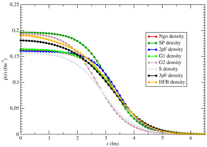
Figure 1 The changes as a function of distance (r) of Ngo, SP, 2pF, G1, G2, S, 3pF, and HFB density distributions in a linear scale.
Table II The rms radii of Ngo, SP, 2pF, G1, G2, S, 3pF, and HFB density distributions as compared with the literature.
| Density distribution | rms radii (fm) |
| Ngo | 3.290 |
| SP | 3.033 |
| 2pF | 3.155 |
| G1 | 3.297 |
| G2 | 3.243 |
| S | 3.251 |
| 3pF | 3.236 |
| HFB | 3.168 |
| Literature | 3.263(2)a, 3.323b, |
| 3.245 ± 0.032c | |
| 3.244 ± 0.018d 3.26e |
a Determined via Ref. [26].
b Determined via Ref. [27].
c Determined via Ref. [28].
d Determined muonic x-ray value [29].
e Determined via Ref. [30].
The imaginary potential parameters have been studied to produce results in good agreement with the experimental data. Although it is very difficult to study on the same potential geometry for different reactions and different density distributions, this method has been preferred in our study. This is because both global equations of the imaginary potential depths and better physical inference are to be presented. For this aim, W 0, r w and a parameters which define the Woods-Saxon potential have been determined by using the following processes; i) r w parameter is determined by varying at 0.1 and 0.01 fm interval at fixed W 0 and aw values, ii) aw parameter is determined by varying at 0.1 and 0.01 fm interval at fixed W and r values, iii) W parameter is obtained for fixed r w and a w values. Thus, r w and a w values have been taken as 1.30 fm and 0.41 fm, respectively.
In our study, we have divided our discussion as the reactions with light, medium, and heavy mass targets. In this context, as for light and light-medium target samples, we have analyzed 32S + 12C reaction at E = 110 MeV, 32S + 27Al reaction at E lab = 100 MeV, 32S + 40Ca reaction at Elab = 100 MeV, 32S + 48Ca reaction at Elab=83.3 MeV, and 32S + 48Ti reaction at E lab = 160 MeV. In Fig. 2 we present the elastic scattering cross sections for 32S + 12C and 32S + 27Al reactions, and in Fig. 3 for 32S + 40Ca, 32S + 48Ca, and 32S + 48Ti reactions. Besides, we have calculated the χ 2/N values for each density distribution, and have listed them in Table III. The 3pF density for 32S + 12C reaction and the SP density for 32S + 27Al reaction are slightly better than the other densities.
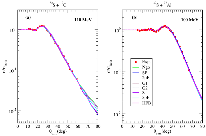
Figure 2 The elastic scattering cross sections calculated by using Ngo, SP, 2pF, G1, G2, S, 3pF, and HFB densities of 32S projectile for (a) 32S + 12C at E lab =110 MeV, and (b) 32S + 27Al at E lab =100 MeV. The experimental data are taken from Ref. [31, 32].
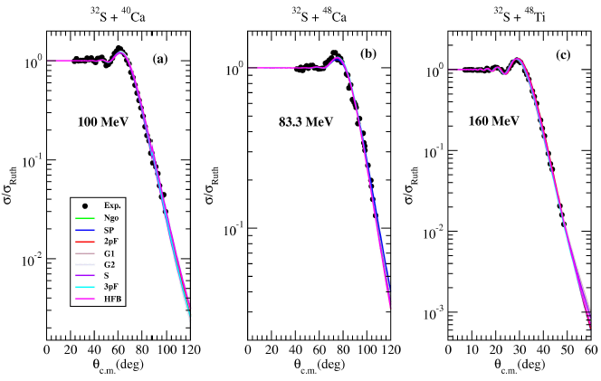
Figure 3 Same as Fig. 2, but for (a) 32S + 40Ca at E lab = 100 MeV, (b) 32S + 48Ca at E lab = 83.3 MeV, and (c) 32S + 48Ti at Elab = 160 MeV. The experimental data are taken from Ref. [33, 34].
Table III The χ2/N values calculated for Ngo, SP, 2pF, G1, G2, S, 3pF, and HFB density distributions.
| Target nucleus | Elab (MeV) | (χ2/N)Ngo | (χ2/N)SP | (χ2/N)2pF | (χ2/N)G1 | (χ2/N)G2 | (χ2/N)S | (χ2/N)3pF | (χ2/N)HFB |
| 12C | 110 | 0.26 | 0.22 | 0.25 | 0.25 | 0.15 | 0.15 | 0.12 | 0.20 |
| 27Al | 100 | 0.16 | 0.07 | 0.14 | 0.14 | 0.14 | 0.12 | 0.15 | 0.15 |
| 40Ca | 100 | 0.42 | 0.85 | 0.69 | 0.64 | 0.68 | 0.44 | 0.53 | 0.81 |
| 48Ca | 83.3 | 0.33 | 0.32 | 0.40 | 0.34 | 0.35 | 0.36 | 0.40 | 0.39 |
| 48Ti | 160 | 0.28 | 0.38 | 0.32 | 0.36 | 0.25 | 0.25 | 0.18 | 0.12 |
| 58Ni | 97.3 | 0.62 | 0.37 | 0.52 | 0.53 | 0.55 | 0.52 | 0.54 | 0.62 |
| 63Cu | 168 | 1.37 | 1.41 | 1.40 | 1.37 | 1.40 | 1.42 | 1.43 | 1.41 |
| 64Ni | 150 | 1.73 | 1.00 | 0.97 | 1.53 | 1.47 | 1.51 | 1.53 | 1.00 |
| 76Ge | 178 | 0.58 | 0.47 | 0.34 | 0.56 | 0.51 | 0.52 | 0.37 | 0.39 |
| 96Mo | 180 | 0.53 | 0.29 | 0.23 | 0.60 | 0.45 | 0.61 | 0.34 | 0.43 |
| 100Mo | 180 | 4.20 | 0.44 | 1.01 | 4.77 | 3.08 | 2.94 | 1.17 | 1.83 |
As regards medium mass target reaction samples, we have calculated the elastic scattering cross sections of 32S + 58Ni reaction at Elab=97.3 MeV, 32S + 63Cu reaction at Elab=168 MeV, 32S + 64Ni reaction at Elab=150 MeV and 32S + 76Ge reaction at Elab=178 MeV. We have compared the theoretical results and the experimental data in Fig. 4. For 32S + 58Ni reaction, it has been observed that the SP density is better than the others while the density distributions investigated are in good agreement with the data. The Ngo and G1 densities for 32S + 63Cu reaction, the 2pF density for 32S + 64Ni reaction, and the 2pF density for 32S + 76Ge reaction are slightly better than the other densities.
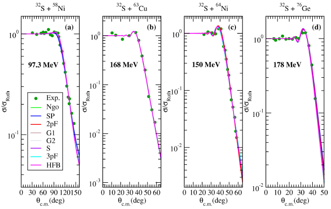
Figure 4 Same as Fig. 2, but for (a) 32S + 58Ni at Elab = 97.3 MeV, (b) 32S + 63Cu at E lab = 168 MeV, (c) 32S + 64Ni at E lab =150 MeV, and (d) 32S + 76Ge at E lab = 178 MeV. The experimental data are taken from Ref. [35-38].
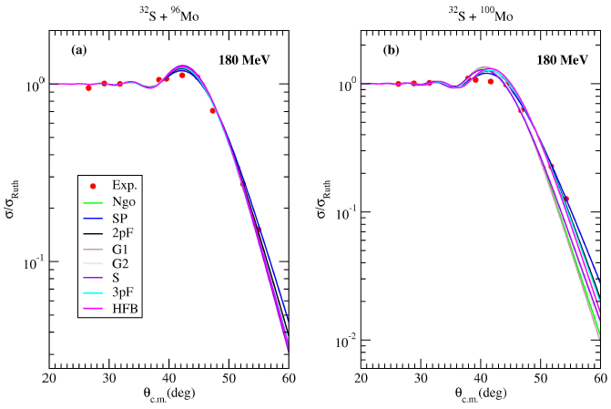
As for heavy target nucleus samples, we have calculated the elastic scattering cross-sections of 32S + 96Mo reaction and 32S + 100Mo reaction at Elab = 180 MeV. We have displayed the theoretical results in Fig. 5. For 32S + 96Mo reaction, we observe that the results of SP and 2pF densities are highly consistent with the data. We notice that the results of 2pF density distribution are better than the results of other densities. For 32S + 100Mo reaction, we notice that density distributions generally exhibit unstable behaviors with each other. However, it has been found that SP density distribution is quite compatible with the experimental data from the comparison of all density distributions.
4.2. Interpretation of normalization constant, reaction cross-section and volume integrals
The normalization constant (N R ) is a parameter used in the double folding model to increase the agreement between experimental data and theoretical results. The default value of this parameter is 1.0. However, the deviation from this value may be due to either uncertainty or peculiarity of experimental data or the fitting process of theoretical calculations. We display the N R values against E/A P for the analyzed reactions by using eight various densities of the 32S nucleus in Fig. 6. The results are sensitive to N R constant, and the N R value has been found to be around unity in heavy nucleus reactions. The results for the medium, heavy targets are very sensitive to the value of N R , and the deviation is high, especially in 32S + 63Cu reaction. One of the reasons can be due to the study performed by using the same potential geometry for all density distributions and reactions.
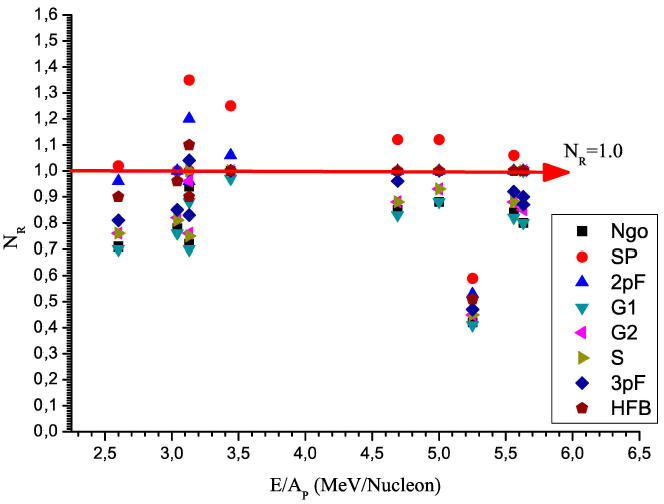
Figure 6 The normalization values (N R ) for the calculations with Ngo, SP, 2pF, G1, G2, S, 3pF, and HFB densities versus E/A P .
The real (J v ) and imaginary (J w ) volume integrals for eight different density distributions have been calculated, and the changes of volume integrals against E/A P are displayed in Fig. 7. The largest J v values have been obtained for the SP density, and the smallest J v values for the G1 density. One of the main reasons for this fact is that the N R values obtained according to the SP density are larger than those obtained according to other densities, whereas the values obtained according to the SP density are larger than those obtained according to other densities, whereas the N R values obtained values obtained according to G1 density are smaller than those obtained according to other densities. Anyway, the J v values of other densities are closer to each other. On the other hand, the imaginary potential parameters are effective on J w volume integrals. While the J w values of the density distributions are generally close to each other, in some cases, they vary according to the values of the imaginary potential parameters.
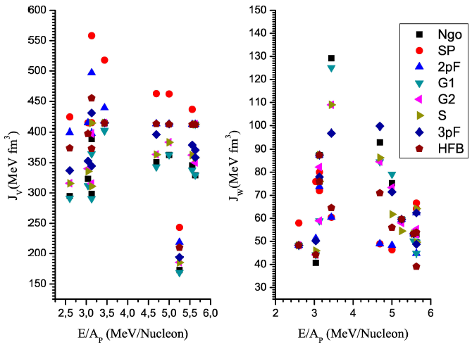
Figure 7 The real and imaginary volume integrals for the calculations with Ngo, SP, 2pF, G1, G2, S, 3pF, and HFB densities versus E/A P .
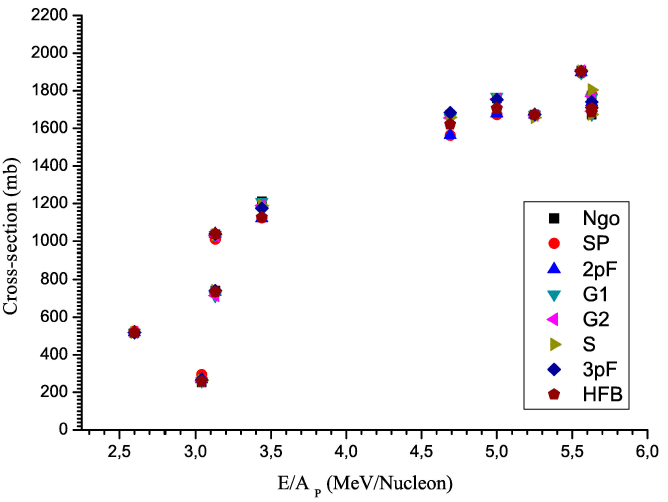
The reaction cross-section (σ R ) is one of the important parameters sought in the reactions analyzed. In this context, cross-section values close to each other for different optical model calculations can be an indication of the suitability of the fitting process applied to the experimental data. The σ R values of all the reactions and for each density distribution are given as compared in Table IV, and are plotted as a function of E/A P in Fig. 8. We can remark that the σ R values obtained for different densities are in agreement with each other.
Table IV The cross-sections (in mb) obtained for Ngo, SP, 2pF, G1, G2, S, 3pF, and HFB density distributions.
| Target nucleus |
Elab (MeV) |
σNgo (mb) |
σSP (mb) |
σ2pF (mb) |
σG1 (mb) |
σG2 (mb) |
σS (mb) |
σ3pF (mb) |
σHFB (mb) |
| 12C | 110 | 1212 | 1124 | 1121 | 1208 | 1189 | 1189 | 1174 | 1126 |
| 27l | 100 | 1036 | 1010 | 1039 | 1034 | 1029 | 1034 | 1039 | 1038 |
| 40Ca | 100 | 743 | 740 | 734 | 714 | 715 | 743 | 741 | 735 |
| 48Ca | 83.3 | 517 | 527 | 520 | 518 | 518 | 519 | 518 | 520 |
| 48Ti | 160 | 1759 | 1672 | 1679 | 1768 | 1755 | 1751 | 1752 | 1706 |
| 58Ni | 97.3 | 254 | 295 | 269 | 260 | 260 | 262 | 266 | 259 |
| 63Cu | 168 | 1672 | 1671 | 1672 | 1672 | 1668 | 1657 | 1673 | 1672 |
| 64Ni | 150 | 1672 | 1563 | 1564 | 1656 | 1655 | 1658 | 1683 | 1621 |
| 76Ge | 178 | 1906 | 1893 | 1898 | 1895 | 1905 | 1905 | 1903 | 1903 |
| 96Mo | 180 | 1672 | 1712 | 1707 | 1673 | 1691 | 1674 | 1710 | 1686 |
| 100Mo | 180 | 1775 | 1780 | 1738 | 1763 | 1770 | 1804 | 1739 | 1704 |
4.3. New and global analytical expressions of imaginary potential depths
Different theoretical models are used to explain the experimental data of nuclear reactions. For this, it is necessary to identify suitable potentials that well define the colliding system. In this context, the optical model is quite valid in explaining the different nuclear interactions. The potential of this model consists of two parts, real and imaginary. In our study, real potential has been obtained with the double folding model. To determine the imaginary potential of the 32S nucleus, new and global analytical expressions are proposed by using the elastic scattering results of different nuclear interactions and density distributions. Thus, these equations can be used as input to the analysis of different reactions. The expressions are formulated as
where E is the incident energy, Z T is an atomic number of targets, and A T is mass number of targets.
5. Summary and Conclusions
Our study has been carried out in two steps. In the first one, elastic scattering cross-sections of the 32S projectile from 12C, 27Al, 40Ca, 48Ca, 48Ti, 58Ni, 63Cu, 64Ni, 76Ge, 96Mo, and 100Mo target nuclei have been calculated at various incident energies. For this purpose, eight density distributions of 32S have been used. The theoretical results have been compared with both each other and experimental data. It has been observed that the density distributions examined in our study have given a general agreement in explaining the experimental data. Additionally, Ngo, SP, 3pF, and HFB densities for light mass target reactions, Ngo, SP, 2pF, and G1 densities for medium mass target reactions, and 2pF and SP densities for heavy mass target reactions are more suitable than other density distributions.
In the second step, the imaginary potential for each density distribution has been obtained by means of the potential parameters used in the 32S elastic scattering calculations. These analytical expressions vary depending on the incident energy of the projectile, the atomic number, and the mass number of the target nucleus. Thus, these equations will be useful in the analysis of reactions concerning 32S nuclei such as elastic scattering, inelastic scattering, transfer reations with both broadly different target nuclei, and incident energies.

