


 nueva página del texto (beta)
 Inglés (pdf)
 Artículo en XML
 Referencias del artículo
 Enviar artículo por email
 Citado por SciELO
  Similares en
SciELO
Similares en
SciELO 
 Permalink
1. Introduction
Percolation theory is a general mathematical theory of transport and connectivity in random complex systems. Percolation is a random process developed from the observation of connectivity between microscopic elements and their effects on macroscopic properties [1]. Percolation looks for a trajectory between the porosity of the medium in a random way, in this mode the fluid crosses the medium from one end to another. The fluid can be a liquid, steam, heat flow, electric current [2], infection or any fluid or property that can move through a porous medium. For example, water on the ground under the action of gravity, sewage treatment plants. Currently, different resistant and low-cost materials are being developed where the material must be light enough, but with a degree of porosity that does not allow liquids to seep through it. Contrary to the manufacture of membranes or materials, that filters fluids in order to eliminate impurities [3]. In this work, we study the percolation in nano-structures [4-7] composed of nano-particles (N - P) such as carbon-gel glucose (AG - CNT) [8] which vary from a size of 1 nm to nano-particles of SiO2 with a size of 100 nm [9]. In this work, we apply a porosity level in a simulated material to know if there is percolation in the material. In Fig. 1, the simulation of a porous material is shown on a cubic grid of size L = 10 with the value of L × L × L = 1000, comprising a grid of the size of 100,000 nm3.

2. Probability and critical probability “Pc”
For a 3D grid G, we use pores of various sizes [12]. To generate the radii of the pores we use a normal distribution, see Eq. (1), with μ r = 0.5 and σr = 0.2 in the simulated grid where r is normalized to the typical system size. Here P is the probability of pores that were generated in the system. The number of pores is determined by the level of porosity called probability P in the system, the larger the probability P in the system.
The critical probability known as Pc in a material is referred to as the Probability P necessary to achieve percolation in a material.
The critical probability in a material is referred to as the probability P necessary to achieve percolation in a material. We can assign P a value from 0 to 1. For each position of the array, random values were assigned in a range of 0 to 1 [13], where we associated this value with the level of porosity, the conditions to generate a pore are as follows:
where G is the grid of the porous material, i, j, and k are the indexes where the pore P o is found and P is considered the level of porosity (PL) that is assigned to the material. If the value of the position of the array is 1, there will be a pore with an assigned radius, otherwise it will not exist. The pore size is determined by its radius r, which is generated randomly with a value between 1 ≥, and r ≤ 100 nm [8,9], where 100 nm is the maximum pore size for our case study. We simulated pores of different sizes considering their radius and volume, since these data will provide information on the porosity of the material, in our investigation we determined that materials with pores of different sizes generally exceed the average volume compared to when fixed radii of 50 nm are handled for our case study.
In Fig. 2, we can observe the typical morphology of a pore which has a spherical geometry for our case study has been used too many times by now [15]. To obtain the volume V of the pore, we considered the formula of Eq. (3), and then we made the summation of the volume of all the pores that are in the 3D grid using Eq. (4) to obtain the level of porosity PL.
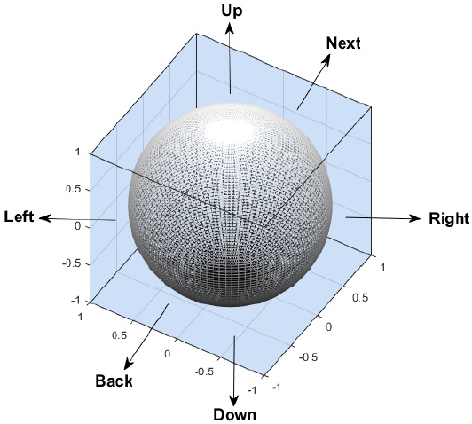
Figure 2 (Color online) Representation of the pore morphology with 3D surface with its 6 nearby neighbors: Up, Down, Left, Right, Back and Next [14,15].
where r is the radius of the pore.
Where L is the length of the cubic grid G. The indices i, j, k are the indices of the grid and V(S) is the total volume of the 3D system.
Since the system generates the pores randomly, there is no certainty of the filtration when there are other configurations where the nearly 6 neighbors are not considered. In this investigation only the pores that have contact with their 6 neighbors are analyzed.
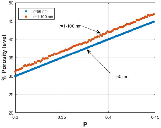
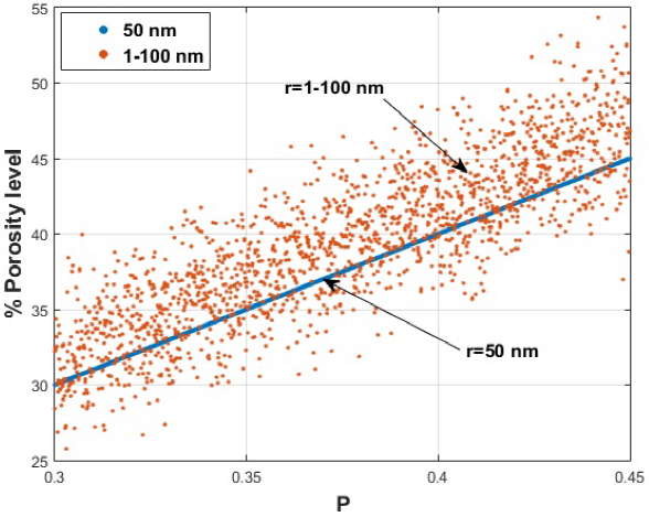
In Fig. 3, we can see several levels of assigned porosity ranging from 30% to 45%, that is to say with a 0.3 ≤ P ≤ 0.45 that the materials can have for a grid of size L = 80, and we observed that the level of porosity in all cases where random radii were assigned (r = 1 - 100 nm) exceeds the level of porosity defined by the user when there are pores of the same radius (r = 50 nm).
We observed in Fig. 3, that the blue line represents pores of fixed radius r = 50 nm with a uniform distribution to the probability P, the red line represents the pores of random radius. We can observe that the level of porosity is higher when there are random radii (r = 1 - 100 nm), that is why its porosity is altered, and the same P distribution is not followed; however, it is altered above the common probability and this causes a greater porosity in the material. If the level of porosity is altered its critical probability Pc is also altered.
3. Cluster and percolation
When one or more pores are large enough to join with their neighboring pores, it will form gaps or spaces that create a long cluster that crosses the material [16], called the percolation cluster or infinite cluster [17]. This depends on the number of pores that exist in the system [18], if there are more pores, infinite clusters are more likely, remembering that the number of pores that can exist in the simulated grid is determined by the probability P.
In Figs. 4 and 5, we see examples of systems with different assigned probabilities [19]. For the first case, P = 0.45 and the second with P = 0.271, both simulated in an array of L = 80. In Fig. 4, we observe that there is percolation in the material, reaching a height of 80, while in Fig. 5 only the clusters that are formed reach a maximum height not greater than 40.
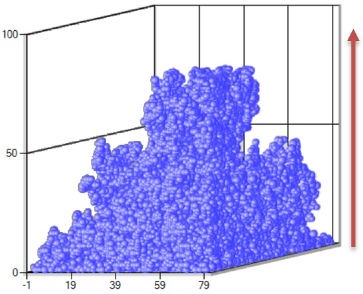
Figure 4 (Color online) Simulated percolation cluster in a three-dimensional array of dimension L = 80, with Probability P = 0:45. The red arrow indicates the direction of the filtration cluster.
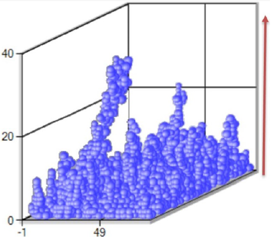
Figure 5 (Color online) Cluster of the same size L = 80 as in Fig. 4 but with probability P = 0:271:
A second important factor for the generation of clusters and infinite clusters, apart from the probability P, is the radius of the pore, since if the radii of the pores are large enough to reach the radius of the neighboring pore, there will be contact between them to form an infinite cluster. The literature [20,21] shows us that for uniform radii with half the diameter d of the pore, the radius r = d/2 is the necessary value to be able to have contact between its close neighbors. The critical probability Pc for pores of uniform radius is approximately 0.311, but nevertheless for random radii with different sizes this value may be altered.
The objective of our research is to study the behavior that nanostructures present when their pores have uniform radius or random radius, and how this property affects the critical probability Pc in the nanostructures. In this study, the infinite cluster cannot exceed the height of the system since the pores are only generated within the 3D model that contains them, although there are other physical phenomena other than filtration that can exceed the system, but those are not addressed in this work. The first step is to generate random radius pores, where the sum of their radii must necessarily be greater than or equal to 1 to have any contact.
In order to create an infinite cluster that, in passing to the percolation, it is necessary to have several pores that have contact with their neighboring pores; a pore in a 3D grid can have 6 nearby neighbors , those that are located up, down, to the left, to the right, back and in next of it (see Fig. 2).
To determine the contact between the pores we must validate that the radius r of the pore that is being evaluated with any of its 6 nearest neighboring pores, in this, there may be some contact C [22]. Taking into account that the pore evaluated in position G[i, j ,k] contains the value of the radius r of the pore with the indexes i, j ,k in array G, the neighboring pores are: next[i, j ,k + 1], back[i, j ,k - 1], up[i, j + 1, k], down[i, j - 1, k], right[i + 1, j, k] and Left[i - 1, j, k].
Equation (5) is used in our investigation in order to obtain the sum of the radii of the evaluated pore G[i, j ,k] and its neighboring pore that is below it G[i, j - 1, k].
where i, j ,k (i = rows of the array, j = columns, k = layer) are the indexes of the array that contain the radius of each pore and C is the distance of the sum of the radii that will define the contact between two pores.
This same procedure will be carried out with the 5 remaining neighbors: next, back, up, right and left. If at least for some of the 6 neighbors of the evaluated pore the following condition is met: C ≥ 100 nm, then the evaluated pore is considered to form the cluster in the 3D grid, otherwise it is neglected and is not considered for creating the cluster.
In Fig. 6 (a), an ideal contact is shown when the radii are uniform with a radius of r = d/2 but nevertheless in real physics any porous material has a non-uniform pore distribution, more similar to Fig. 7 (b), where neighboring pores differ in pore size and radius. In Figs. 7(a) and 7(b), the two important cases are considered when random radii are applied, since the case of Fig. 7 (a) is difficult to find in nature.
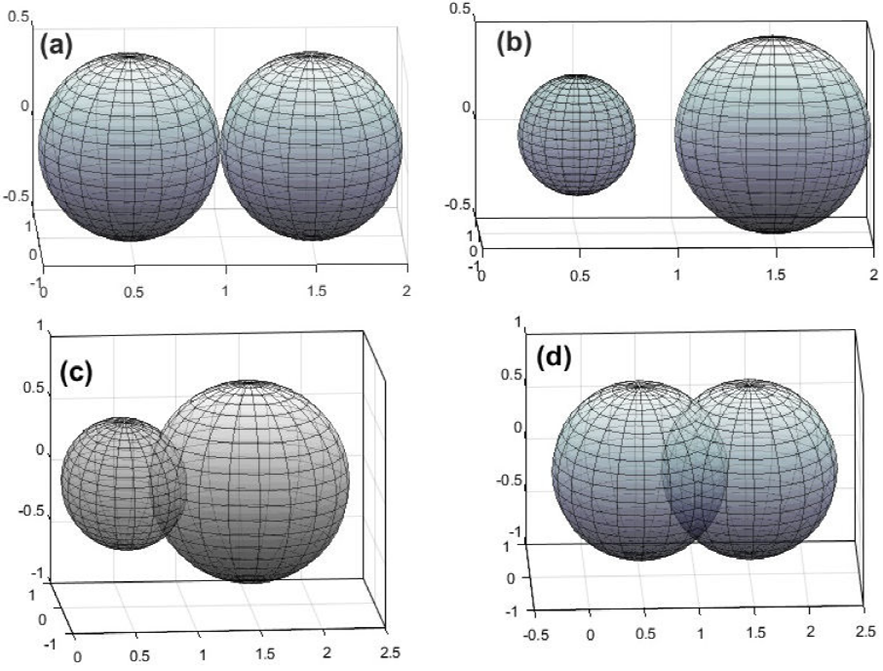
Figure 6 (a) Contact between 2 pores with equal radii; (b) Two pores with random radii are shown, where there are no contact between them, since the radius of the first pore is much smaller than the radius of the second pore and is not large enough to have contact with its neighboring pore.
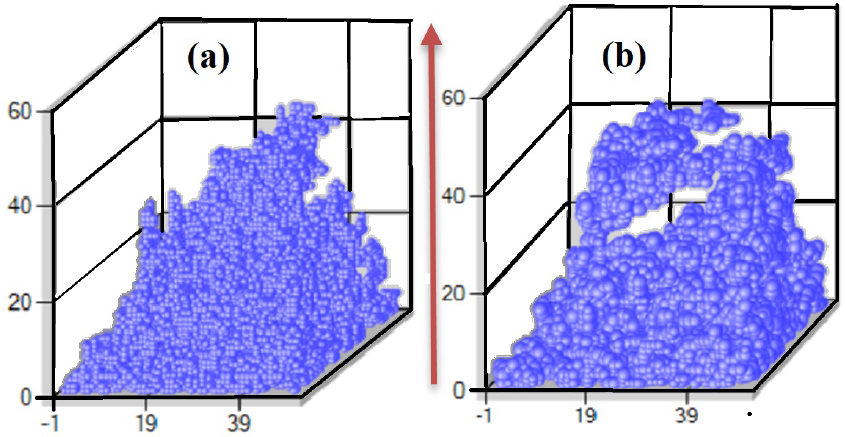
Figure 7 (Color online) We observe in images (a) and (b) two infinite clusters that can conduct the fluids in the material with a filtration orientation from the bottom up. We can observe a greater porous granularity in the image (b) with pores of variable radius, while in the image (a) we observe uniform pores.
In Figs. 6(a), (c), and (d), we find safe contacts between neighboring pores and the contact condition C is met [14], but the case in Fig. 6 (b) is excluded since there is no contact.
In the case of Fig. 6 (b), we consider that the possibility of forming clusters in the material decreases, since this condition did not previously exist and it was just enough to have a neighboring pore with a uniform radius r = d/2 as shown in Fig. 6 (a), with which the contact was safe. We made a comparison to obtain the differences between the critical probabilities when there are uniform radii and random radii, in Fig. 7 (a) there can be seen pores with uniform radii of 50 nm equivalent to r = d/2, and in Fig. 7 (b) pores with different radii sizes ranging from 1 nm to 100 nm can be seen; the grid size for these examples is L = 60 (6,000 nm) and with a probability of P = 0.45 (45% porosity) for both cases.
We simulated pores of different sizes considering their radius and volume, since this data will provide information on the porosity in the material. In our investigation, we observed that materials with random radius pores generally exceed the average volume compared to when fixed radii are handled.
4. Results
We generated several tests in a probability range P = 0.3 to P = 0.5 (30% to 50% porosity) for random pores to be able to find the critical probability in a 3D system, considering a grid size of L = 100 (equivalent to 100,000,000 nm3), where we calculated the height of the infinite cluster. If the infinite cluster reaches the maximum height of the grid L = 100, then there will be percolation and the material can be considered as a porous material. In our tests, we considered N = 1000 calculations distributed in a probability range P = 0.3 to P = 0.5. In Fig. 8, we can observe the behavior of these values and the point where the critical probability form infinite clusters. In this graph, the heights for each level of porosity or probability P are shown.
The critical probability in the case of Fig. 8, is obtained when the bars that represent the maximum height of the cluster for each probability reach the maximum height of the grid, for this case L = 100 is reached at the point Pc = 0.4329.
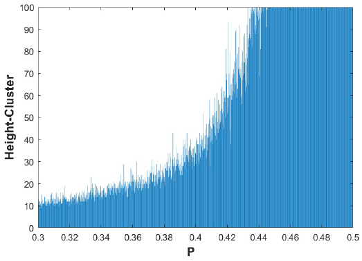
Figure 8 (Color online) Results for critical probability. 1000 calculations were distributed in a probability range or porosity level of 0.3 to 0.5. Each bar represents the value of the cluster height of an assigned probability in the range of 0.3 to 0.5, for this value of L = 100 the Pc is 0.4329.
In Fig. 9, we observed the number of pores in the cluster that are formed for each test performed, we can see that the more likely the system is assigned, the more pores will be generated in the material. If the probability is small, the material will be poorly porous, but if the probability is large then the material will increase its porosity level; this relationship can be seen in Fig. 9, where each point represents the number of pores by probability P, in a range of 0.3 to 0.5. We can observe a distribution of small pore generation to the point of probability P = 0.4, where the level of porosity increases rapidly.
The approximate execution time to perform this test was approximately 9 minutes and 4 seconds for the calculations shown in Fig. 9.
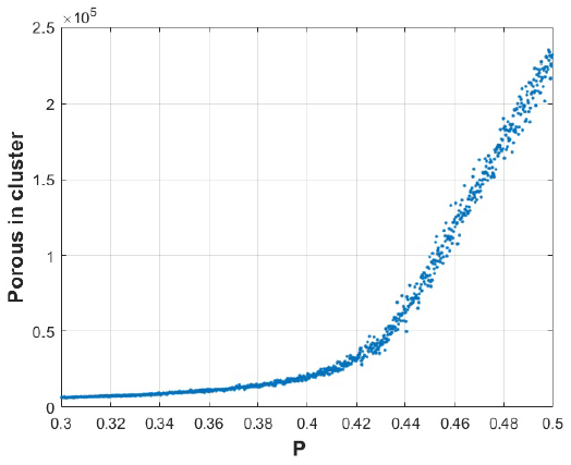
Figure 9 (Color online) A porosity distribution of 30% to 50% (P = 0:3 to 0.5) is shown, each point represents the number of pores that were generated in the simulated 3D system.
In Fig. 10, we observed the time relationship for each test calculated. The results of these calculations for our numerical simulation were performed on a Dell computer with Intel (R) Core (TM) i7-6700HQ 64-bit processor, at 2.60 GHZ with 8 GB of storage RAM.
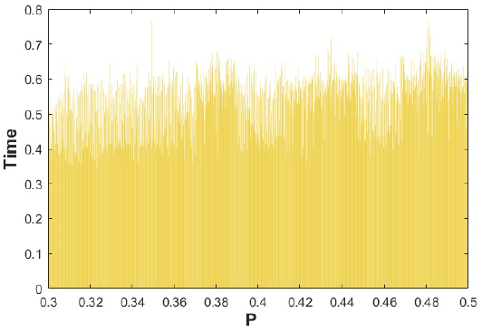
Figure 10 (Color online) The time in milliseconds for each calculation is shown in a probability distribution P = 0:3 to P = 0:5, and a number of calculations N = 1000, having an average time for each of approximately 4.5 milliseconds.
In this work a range of grid sizes from L = 5 (500 nm) to L = 100 10,000 nm) was studied, excluding the behavior of larger arrays to these measurements. We performed several calculations for different grid sizes to obtain the critical probability, starting from a small grid to a large grid, we can observe this relationship in Fig. 11, where the critical probability values that are reached for sizes L = 5 are shown (500 nm) to L = 1000 (10,000 nm).
From Fig. 11 we observed that the curve for fixed radius pores r = 50 nm, critical probabilities Pc greater than those of random radius pores are reached when the sizes of the grid L are small, approximately when L = 10 (1000 nm) to L = 40 (4000 nm), but for larger grids containing pores of random radius the critical probability exceeds the critical probability Pc of the pores with fixed radius.
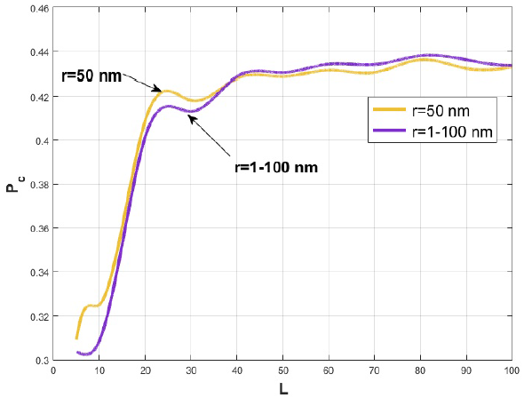
Figure 11 (Color online) The behaviors for random radii with radius 1 ≤·r ≤·100 nm and fixed radii with (r = 50 nm) are shown.
From Fig. 12, we can see that there is greater dispersion of porosity levels when the simulation grid is small (L = 10), and when the pores radii are random, there are lower porosity levels than the fixed radii. Contrary to the opposite case of Fig. 3 with size L = 80, where the pores of random radius are larger than those of fixed radius.
5. Conclusions and future works
The contribution of this work is the study of the percolation of random radius materials in the pores present in nanostructures. For cases where there are small grids, the porosity levels in the material with random radii may be lower and below that of the fixed radii as shown in Fig. 12, which is why there may be small changes in the critical probability, as shown in Fig. 11, where we observe that when the grids have a small dimension they exceed the Pc of the random radii, but as the array becomes larger the value of the Pc for random radii exceeds the Pc of the fixed radii.
We can conclude that the parameter L, (grid size) can affect the porosity and therefore the generation of infinite clusters when random radii are studied, the dispersion of the porosity with random radius varies above and below that of the pores of fixed radii when the grids are small, but for large grids it slightly exceeds the porosity of the fixed radii. Random radius nanostructures are more porous and their critical probability increases when the grid sizes exceed the measurements of L > 40. Small grids L < 40 with pores of random radius may be less or more porous than those of fixed radius altering their Pc.
In this investigation, percolation is modeled considering spherical pores, which provides an approximation to the phenomena of percolation in porous materials, so that the morphology and complexity of each material provide an infinite range of porous formations, which opens the possibility of future research.

