1. Introduction

A derivative of a function at some point characterizes the rate of change of the function at this point, that is, the ordinary derivative is local. Any process that changes over time or with space can be described by an ordinary differential equation, in partial derivatives or by a system of equations, ordinary or partial. For example, Newton’s law of cooling states that the rate of change of temperature of the body is proportional to the difference between the temperature of the body and that of the surrounding medium [¹]. Then, solving the given differential equation, we can predict the behaviour of the temperature of the system. However, the real description of the propagation of the temperature can be quite complex depending on the heat source and of the internal structure of the material, see Fig. 1, and this is where the ordinary calculation stops working and gives rise to the other possible derivatives, such as fractional or conformable derivatives. Fractional calculus (FC), involving derivatives and integrals of non-integer order, is the natural generalization of classical calculus; during recent decades has become a powerful and widely used method for better modeling and control of processes in many areas of science [²-⁶], engineering [⁷-¹⁰], and financial economics [¹¹]. The fractional derivatives are nonlocal operators, because they are defined through integrals. Fractional derivatives satisfy the property of linearity; however, properties (such as the product rule, quotient rule, chain rule, Rolle’s theorem, mean value theorem and composition rule, etcetera) are lacking in almost all fractional derivatives. To avoid these difficulties, in [¹²], it was proposed an interesting idea that extends the ordinary limit definitions of the derivatives of a function, called conformable fractional derivative, from now on, we will only call it a conformable derivative (CD) because is a local operator. This CD has attracted the interest of researchers, as it seems to satisfy all the requirements of the standard derivative. Also, computing using this new derivative is much easier than the fractional derivative. As expected, there are many works related to this derivative, for example [¹³-²⁰], to name a few.

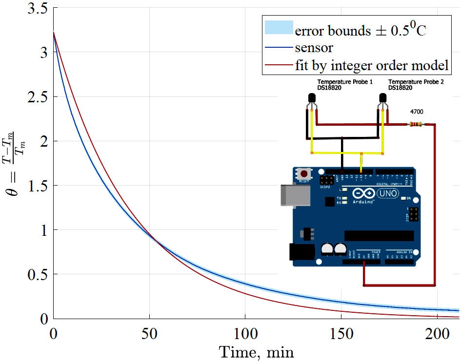
FIGURE 1 Experimental data fitted by integer order model Eq. (4), with the best value of k =0.02438 1/min. 

Recently in [²¹], the conformable derivative was applied to Newton’s law of cooling, having as a solution the Kohlraush stretched exponential function. In that case, a closed expression for the convection coefficient k, depending on the fractional order derivative 0 < γ ≤ 1, was obtained.

In this work, we performed an experimental setup to verify the effectiveness of the conformable derivative applied to fractional Newton’s law of cooling. It is shown that the theoretical solution given in [²¹] coincide with the experimental data when the fractional order is γ = 0.77269 and k = 0.018765.

2. Conformable Newton law of cooling

Let f:[0,∞)→R be a function. Then the γ-th order conformable derivative of f is defined by [¹²] as

for all t > 0 and 0 < γ ≤ 1. This expression is not the only possible [²²,²³].

When γ = 1 from (1), we obtain

The CD is easily computed, but it is not conformable at γ = 0. The differentiation properties of this conformable derivative are analogous to the properties of the ordinary derivative, and the relation

is fulfilled [¹²]. On the other hand, Newton’s law of cooling says that under certain circumstances the rate of change of temperature of a body is proportional to the difference between the temperature of the body and that of the surrounding environment [¹], as long as the temperature difference is not very large. The above is described by the equation

where T(0) = T ₀ is the initial temperature of the body, T _m is the temperature of the medium considered constant, and k is the convection coefficient. The coefficient k is measured in inverse unity of time, s ⁻¹. The Eq. (3) has an analytical solution in the form

In the previous work [²¹], to maintain the homogeneity of the fractional differential equation for Newton’s law of cooling, the ordinary derivative operator was changed by a fractional one, in the following way,

substituting in (3), we have the corresponding fractional differential equation of order γ,

Solutions of this fractional equation using other fractional derivatives have been reported in [²⁴].

However, with these fractional derivatives, it is not easy to calculate the convective coefficient k. Due to this, in [²¹] was applied the conformable derivative [¹²]. For this, we take into account the expression (2), we have

Substituting this time-fractional conformable transform in (6), we obtain an ordinary differential equation

This equation has the particular solution [²¹],

So, in the case of CD the Newton’s law of cooling has the stretched exponential function (or Kohlrausch function) of order 0 < γ ≤ 1 as a solution. This function has many applications in science: it fits many relaxation processes in disordered and molecular systems [²⁵-²⁷], this is due to the free parameter γ in the exponential function. For a given time τ and temperature T ₁ we can compute, in a closed form, the conformable convective coefficient

unlike the results obtained in [²⁴] using the RiemannLiouville and Caputo fractional derivatives, where does not possible to obtain.

3. Data acquisition

Cooling experiments were performed using 300 ml of hot water in an isolated ceramic cup. The temperature was measured using a data acquisition system based on two DS18B20 temperature digital sensors attached to the Arduino board (AB), model UNO-R3. One of the sensors was kept fully submerged in the center of hot water volume. The other one was placed outside to monitor the ambient temperature.

The waterproof sensor DS18B20 provides data in digital form, with an accuracy of ±0.5°C and a maximum resolution of 6.25×10⁻² °C without the need for any analog-to-digital conversion or calibration. The ensor comes with three wires: the red one is connected to 5 V, the black one is connected to ground, and the yellow one is connected to a digital input pin of the AB (pin 10 in our case). For these sensors, a pullup resistor R = 4.7 kΩ is needed between the digital input pin and the 5 V source. The connection diagram for the AB (created with Fritzing) is shown as an inset in Fig. 1.

The communication between the sensors and the AB is implemented in three steps:

The Arduino-script we used has two parts, the setup subroutine and the loop subroutine using the OneWire library into the Arduino Integrated Development Environment (IDE).

4. Data Processing and Results

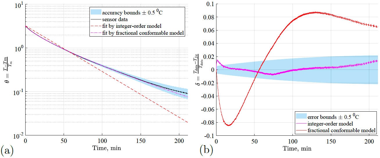
The temperatures are registered with an average time step ∆t = 28.45 ms for almost 3.5 hours. The measured average ambient temperature is T _m = 20.9147°C. Then these data have been fitted by both integer (4) and conformable (9) models. The χ ²-criterion has been applied when fitting experimental data. Results in Fig. 2(a) shows a drastic divergence of integer model from experimental data. However, the conformable model provides an ideal fitting, as we can see from the quantitative analysis of residuals in Fig. 2(b). The conformal model provides results within experimental accuracy in the whole range of measurements, and thus, they are indistinguishable from the measured data.

FIGURE 2 (a) Fitting by conformable fractional-order model. (b) Best result is for γ =0.77269 and corresponding k =0.018765 1/min. 

5. Conclusions

The main aim of this work was to compare the theoretical results obtained in [²¹] with the real data obtained experimentally. We conclude that even in a very simple case, as is Newton’s law of cooling, the integer order differential equation can not correctly predict the behavior of the system. In this work, it was shown that the solution (9) of the conformable differential equation (8) fits very well with the experimental data when γ = 0.77269 and k = 0.018765. Unlike other fractional formalisms [²⁴], the conformable derivative has an analytical solution very similar to the ordinary case, and fits very well with the experimental data; this is due to the free parameter 0 < γ ≤ 1. This is interesting since the conformable derivative contains the same differentiation rules as the ordinary derivative, which does not contain the fractional derivatives known until today.

We hope that the way of analyzing the fractional differential equations using the conformable fractional transform (7) will be helpful in solving fractional equations that represent more complex systems.