


 nueva página del texto (beta)
 Inglés (pdf)
 Artículo en XML
 Referencias del artículo
 Enviar artículo por email
 Citado por SciELO
  Similares en
SciELO
Similares en
SciELO 
 Permalink
1. Introduction
Thr scale factor determines the evolution of the universe. At the initial stages, it is closest to its minimum value. At later stages, the scale factor approaches infinity, classically. Here, Table I shows the divergence of various singularities.
The classical cosmological model does not provide detailed information about the dynamics of the universe at the singularity, due to the vanishing scale factor. Particularly, the classical analysis of the singularity does not make sense. The Wheeler-Dewitt analysis and the LQC provides detailed information about Hubble parameter at the initial stages of the universe.
The initial singularity is the mysterious problem from the theoretical standpoint predictions. The classical analysis did not resolve the initial singularity; quantum treatment is required. To analyse the initial singularity. With the help of background-independent resolution, the loop quantum gravity provides a tool to understand the quantum nature of the Big Bang. Time and critical density dependence of the scale factor are determined by loop quantum cosmology. Similarly, pre-Big Bang scenario is characterized by the conformal cyclic cosmology. This confirms the cyclic evolution of the universe. In such resolutions, the conservation of information is required to be understood. In recent days, Penrose expressed his ideas about the confirmation of the existence of Hawking points from previous Aeon, through the CMB radiation [1].
The classical singularity is a mathematical point, in which the cosmological parameters such as energy conditions, pressure, and curvature face divergences [2]. Every classical cosmological scenario avoids the initial singularity. The singularity can be analysed through a quantum mechanical perspective. The quantum mechanical solutions provide the understanding of initial conditions of the universe. Dynamics of the universe is approached with many theoretical models such as Big Bang [3], Ekpyrotic [4], cyclic [5], Lambda CDM [7] and many more. The initial conditions of the universe resemble like quantum mechanical vacuum fluctuations [8]. The Wheeler-Dewitt model was proposed for the quantization of the gravity [9]. It is applied for the quantum analysis of initial stages of the universe.
From such solutions, the universe is said to be created spontaneously from quantum vacuum [10]. The quantum universe that pops out of a vacuum does not require any Big Bang-like singularities [11]. Similarly, such a scenario requires no initial boundary conditions. In contrast to other models, the LQG makes consistent results over renormalization of quantum parameters for quantizing the gravity, to avoid infrared ultraviolet divergences [12]. The Loop Quantum Cosmology resolves the classical singularity and examines the universe quantum mechanically [13]. In LQC, the quantum nature of the Big Bang is analysed [14]. The loop quantum model suggests that at singularity, the quantum universe bounces back as the density approaches the critical level. Hence, the Big Bang is replaced with a Big Bounce iin the loop quantum cosmological scenario [15]. The formation of the quantum mechanical universe from the quantum vacuum is discussed here with the help of the Wheeler-Dewitt theorem. With scale factor quantization, the behaviour of the quantum cosmological constant is also discussed. A timevarying cosmological parameter is proposed to have a consistent value for the cosmological constant, which is currently a need of the hour. The scale factor solutions are discussed for the k = 0 model.
To construct a local supersymmetric quantum cosmological model an alternative procedure is presented in [16]. A superfield formulation is introduced and applied to the Friedmann-Robertson-Walker FRW model. Scalar field cosmologies with perfect fluid in a Robertson-Walker metric are discussed in [17]. Asymptotic solutions for the final Friedmann stage with simple potentials are found in the same work. It also predicts that the perfect fluid and curvature may affect the evolution of the universe. Scalar phantom energy as a cosmological dynamical system is reported in [18]. Three characteristic solutions can be identified for the canonical formalism. Effect of local supersymmetry on cosmology is discussed in [19]. The authors discuss the case of a supersymmetric FRW model in a flat space in the superfield formulation.
The interactions of phantom energy and matter fluid are reported in [20]. Avoidance of cosmic doomsday in front of phantom energy is reported in the same. What will happen for the universe, soon after such singularity is approached? Will Type I singularity stop the evolution of the universe? Will it be the endpoint of all universes? Answers for these questions are discussed in this work. Evolution of the universe is explained by the various cosmological models.
Initially, this work starts with a basic introduction on conformal cyclic cosmology. In the next section, an introduction to phantom energy and dark energy is provided. In the next section, an overview for loop quantum cosmology is discussed. We discuss quantization procedures. In the next section, we analyze the solutions for Wheeler-Dewitt equations. A comparison between Wheeler-Dewitt cosmology and classical supersymmetric cosmology is drawn. In later sections, we provide solutions for non-interacting dark energy which leads to the continued evolution of the universe without approaching the final singularity.
2. Conformal Cyclic Cosmology
The Conformal Cyclic Cosmology (CCC) provides alternative explanations for existing cosmological models [20-22]. The CCC predicts the evolution of the universe as cycles or Aeons. The repeated cycles are referred to as Aeons. Each Aeon starts from a Big Bang and ends up with a Big Crunch. The CCC follows conformal structure over the metric structure. The CCC approaches the initial stages of the universe in a lower entropic state which was higher for the remote part of the previous Aeon [22]. The universe without inflation is predicted by conformal cyclic cosmology. The CCC explains the imbalance between the thermal nature of radiation and matter in the earlier phases of the universe. The suppression of gravitational degrees of freedom is a consequence of remote past Aeon which has low gravitational entropy. Thus the universe is proposed as the conformal evolution over the Aeon. It is possible to cross over the Aeons, due to the conformal invariance of physics of massive particles which survived from past Aeon. The materials of galactic clusters remain as the form of Hawking radiation. Due to the evaporation, massive particles can be available as photons for the future Aeons, after the survival from Big Bang singularity. The cosmological constant Λ is suggested as invariant in all Aeons. In CCC the inflation is said to be absent. The Λ overtakes the inflation, that provides exponential expansion. The CCC is consistent with LCDM [23], without implementing inflation. The CCC does not violate the second law of thermodynamics [24]. The conformal cyclic cosmological model topologically analyses the past and future singularities as surfaces with smooth boundaries. Hence, future and past boundaries are equated with the same kind of topology. Relationship between past and future singularities mainly exist in the scale factor. Though the singularities come under various types, the initial Big Bang and future Big Rip are compared in Table III. This comparison is of interest for of the Big Rip is considered as the end of the evolution of the universe. So the scale factors from Big Bang and Big Rip can be mapped conformally with each other. Comparisons of scale factor from loop quantum cosmology and classical super symmetrical solutions are discussed in this work.
TABLE II Types of singularities.
| Type | Singularity |
| Type 0 | Big Crunch or Big Bang singularity |
| Type I | Big Rip singularity |
| Type II | Sudden future singularity |
| Type III | Future scale factor singularity |
| Type IV | Big separation singularity |
| Type V | ω singularity, little rip pseudo singularity |
TABLE III Strength of singularities is determeined by the various parameters.
| η 0 | η 1 | k | c 0 | Tipler | Królak |
| (−∞,0) | (η 0,∞) | 0, ±1 | (0, ∞) | Strong | Strong |
| 0 | (0,1) | 0, ±1 | (0, ∞) | Weak | Strong |
| 0 | [1, ∞) | 0, ±1 | (0, ∞) | Weak | Weak |
| (0,1) | (η 0,∞) | 0, ±1 | (0, ∞) | Strong | Strong |
| 1 | (1, ∞) | 0,1 | (0, ∞) | Strong | Strong |
| 1 | (1, ∞) | -1 | 1 | Strong | Strong |
| 1 | (1, 3) | -1 | 1 | Weak | Strong |
| 1 | [3, ∞) | -1 | 1 | Weak | Weak |
| (1, ∞) | (η 0,∞) | 0, ±1 | (0, ∞) | Strong | Strong |
Information on the existence of Hawking radiation from previous Aeon can be obtained from Hawking points. Such Hawking radiation obtained from Hawking points might be the remnant of the super-massive blackhole of the previous Aeon. Such existence can be proven by mathematical and experimental solutions such as cosmic microwave background [1]. The conformal cyclic cosmology is theorized with the Aeons. The universe evolves as Aeons. Evolution begins from a singularity grows with exponential expansion, reaches the critical density and then they end up with singularity again. Before proceeding into such mappings, some introduction about fundamental topics are required.
3. Dark energy and Phantom energy
The dark energy is a mysterious form of the energy content of the universe. The equation of state ω determines the acceleration of the universe. From Einstein’s field equations, cosmological constant is proposed for the consequences for the accelerated expansion of the universe [25]. In general, the cosmological constant value is smaller than the expected value from quantum gravity. Though the technical conflicts exist between the theory and experiment, cosmological constant is included in Einstein’s field equations.
The phantom energy has the values of equation of state parameter ω < −1. The phantom energy violates the null energy conditions. The phantom energy is proposed as a candidate for the sustainability of traversable wormholes [26]. Wormholes metric with the dominance of phantom energy is studied in [27]. Symmetric distribution of phantom energy in a static wormhole is also reported. The phantom energy has super-luminal properties. Such properties are similar to those predicted by supergravity or higher derivative gravitational theories [28-30].
In the evolutionary phase of the universe, the singularities can be classified by the diverging parameters. Big Rip singularity appears in a finite time. The finite-time singularity will occur with weak conditions of ρ > 0 and ρ + 3P > 0 in an expanding universe.
A Type I singularity has a scale factor divergence along with the associated to energy density and pressure. Type II singularities are referred to as sudden feature singularities. Divergence of pressure with finite scale factor and energy density occurs. Type III is referred to as big freeze singularity. In Type III energy density and pressure diverge with a finite scale factor. Type IV singularity is referred to as big separation singularity, where energy density pressure and scale factor remain finite, but the time derivative of pressure or energy density diverge. The universe can be extended after it approaches singularities of either Type II or IV, because they are relatively weak. The strong Big Rip singularities is resolved here using loop quantum cosmology. Among these singularities Type zero is experienced by the universe at the earlier stages and Type I is encountered at later times.
Various cosmological singularities are reported in [31]. The scale factor has the following characterization.
where η 0 < η 1 < ...,c 0 > 0
The geodesics are parameterized as
and
with
It has been used for simplicity a constant geodesic motion P and δ = 0 and 1 for null and time like geodesics. For null geodesics δ = 0
If η 0 > 0, the scale factor vanishes at t 0. Hence, there will be either a Big Bang or Big Crunch. If η 0 = 0, then the scale factor will be finite at t 0. A sudden future singularity will appear in the evolution of the universe. If η 0 < 0, then the universe will face Big Rip at t 0. If the cosmological models exist with η 0 ≤ −1, then the null geodesics will avoid the Big Rip singularity. In our solutions, η 0 → (−∞,0), η 1 → (η 0 ,∞), k = 0,±1, and c 0 → (0,∞). Various cosmological singularities [32-34] are reported in Table III.
ω = const is not the only option to obtain an accelerated cosmic expansion. There are dark energy parameterizations that can cross the phantom divided-line with success and also reproduce ω = −1.
TABLE IV Dark energy parameterizations with best fits and σ−distances values using SNe Ia JLA data. Referred from [35].
| Model | Parameterization |
| LCDM |
|
| Linear |
|
| CPL |
|
| BA |
|
| LC |
|
| JBP |
|
| WP |
|
Six bidimensional dark energy parameterizations are studied and tested with available SNe Ia and BAO data [35]. Obtained results are in favour of the LCDM model. Various parameterizations are reported in the same reference. The Friedmann-Raychaudri equation is
where H(z) is the Hubble parameter, G the gravitational constant, and the subindex 0 indicates the present-day values for the Hubble parameter and matter densities. For dark energy
with
For quiessence models, w = const.
Solution of f(z) is therefore,
For cosmological constant, w = −1 and f = 1.
In addition to the simplest models in which the universe contains only cold dark matter and a cosmological constant, class of braneworld models can lead to a phantom-like acceleration of the late universe [36]. This model does not require any phantom matter. The quintessence leads to a crossing of the phantom divide-line w = 1. This model avoids the future Big Rip by decreasing the Hubble parameter.
For w q > −1, a smooth crossing of the phantom divide occurs at a redshift z c that depends on the values of the free parameters Ωm, Ωq and w q. z c is obtained as
For LDGP model w q = −1, the crossing occurs at α = ∞. At a redshift z ∗ > z c, we have ρ eff(z ∗) = 0. Hence, the phantom GR picture of QDGP diverges.
The future Big Rip can be avoided due to the parameters
This shows that ω eff(z) ≥ −1.
For the quantization of the singularity, the basic understanding of quantum geometry is required. The quantum geometric analysis, done via loop quantum geometry is discussed in the next session.
4. Loop quantum cosmology - a brief analysis
The canonical quantum gravitational formalism is based on the quantization of the metric. It attempts to quantize the phase space as a Hilbert space. In canonical formalism, the phase space variables are replaced by operators. But the formalism faces some constraints. There are Hamiltonian, diffeomorphism and Gauss constraints. To solve these constraints, Loop Quantum Gravity is proposed. The model has numerous success in resolving the initial singularity. The model provides background free solutions for the canonical gravity approaches. The Loop Quantum Gravity explains the discreet nature of the spacetime. On cosmological scales, Loop Quantum Cosmology is proposed for the unperturbed evolution of the universe.
Loop Quantum Cosmology is based on the canonical quantum gravitational formalism. The Loop Quantum Gravity does not require renormalization; this makes LQG stand special over other quantization approaches. From canonical quantization, one can expect non zero discrete values for geometric quantities as quantum observables. Hence, the Loop quantization approach provides non zero values for area and volume. Area and volume in LQG are formulated as operators.
The constraints reduce the possibilities of quantization. Setting constraints as c = 0, then the solution of the quantum evolution will be
In general, every cosmological scenario faces singularities during the initial stages of evolution. The initial conditions of the universe possess strong singularity. The initial Big Bang singularity bears high curvatures and energy density divergences. To resolve this singularity conditions, LQC is equipped with the application of LQG theory. LQG attempts to derive non-perturbative and background independent quantization of general relativity. In LQC there is a straightforward link between full theory and the cosmological models, which is in contrast to other cosmological approaches. The full theory of quantum gravity is required to be constructed. The LQC is based on symmetrical reduction. But this methodology faces mathematical problems in full theory. So, current research is happening on symmetrical, non-symmetrical models and their relationships.
In Robertson-Walker metric for a flat (k = 0) homogeneous isotropic universe in Loop Quantum Gravity (LQC) is
with α(t) scale factor and t is the proper time. The effective Hamiltonian in LQC
The details of quantum dynamics are provided by the effective Hamiltonian, and
Where V = α 3 and γ = 0.2375 is the Barbaro-Immirizi parameter [37]. The phase space variable from classical dynamics is
The parameter λ determines the minimum eigenvalue parameter of LQG and the discreteness of quantum geometry [38]. The parameter is denoted as
If the Hamiltonian constraint is vanished
with
the energy density. From the Hamiltonian equation,
This equation can call the modified Friedmann equation as
where the critical density is inferred as
Similarly, the Raychaudhuri equation is also modified with the help of
which holds the conservation law
where the pressure is
Hubble parameter in gravitational Hamiltonian is replaced by the holonomies. They are non linear functions of α and
where v is the mean size units in 3D space and n the number of sections in the region. Implementation of discreteness of quantum geometry results in the dynamics. It depends on the patch size and independent of the number of patches n. Holonomies are represented as
These modified equations express the Ricci flow on FRW background. We may discuss about the curvatures. Invariant form of Ricci curvature will be
From the Eq. (33), it can be observed that the curvature scalar approaches negative values for the chosen parameters such as ρ = ρ crit and ω < −1. Hence Anti-Desitter kind of future universe may appear. Also, the conformal Aeon will face regulated future singularity as AdS like singularity.
Similarly, the Ricci components can be written in terms of lapse function N and scale factor as defined in [40],
The Friedmann equation can be obtained in terms of Ashtekar variables as
where
and
In general, the AdS universe expands eternally. But there exists a maximum cut-off by loop quantum cosmological solutions. Those solutions predict that when the energy density reaches ρ crit then the universe will nucleate future Aeon.
With
as λ → 0 which results in
In LQC, the scalar field is considered as an internal clock. The Hubble distance is defined as
In LQG formalism, the canonical part satisfies
The scale factor is quantized with Ashtekar variables [14] as follows,
Its conjugate momenta is represented as
with
which satisfies
Here,
The holonomy
The metric of an isotropic slice is
Here
To understand the space of metrics or structure tensors, Ashtekar variables are introduced.
Triads can be written as denstized form. That the densitized triads conjugate extrinsic curvature coefficient.
The curvature is replaced with Ashteaker connections.
Ashteaker connections conjugate to triads will be
Hence, the spin connection will be
The spatial geometry is obtained from densitized triads.
An expression for the inverse scale factor is
The inverse scale factor M IJ can be quantized to volume operator [43]. The bounded operator will be
Quantization of the inverse scale factor does not diverge at the singularity. Even though the volume operator diverges approaches to zero, the corresponding inverse scale factor doesn’t approach zero.
There are eigenstates of volume operator
Those results for eigenspectrum and scale factor values are plotted in Fig. 2.
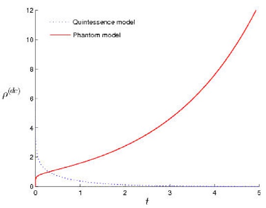
FIGURE 1 Increment of phantom energy over time is shown in the figure. As time increases the phantom energy keep on increases. Referred from [58].

The full Hamiltonian depends upon the patch volume but not the number of patches or the total volume.
5. Wheeler-Dewitt solution for initial scale factor
Wheeler-DeWitt equations attempted to quantize the initial singularity. Like Einstein’s field equation Wheeler-DeWitt equation is also a field equation. The Wheeler-Dewitt approach attempts to quantize gravity by connecting General Relativity and Quantum Mechanics. The Wheeler-Dewitt equation resolves the Hamiltonian constraint using metric variables.
Mini super-space models can be implemented to explain the emergence of the universe [45-47]. Action of mini superspace is defined as
Metric of the mini super-space is defined by
The mini super-space is considered to be homogeneous and isotropic.
and the momentum is
The canonical form of the Lagrangian can be written as
where
The Wheeler-Dewitt theory determines the evolution of the universe. The Hamiltonian is in the form
and
Then the WDWE is changed as [48,49]
Here, K = 0,+1, and -1 for flat, closed, and open bubbles, respectively. The quantum trajectories can be obtained, from quantum field theory and non-relativistic perspectives [45,50]. It is represented as
The inflation occurs for the selected values of p = −2 or 4. The quantum vacuum experiences exponential expansion which is triggered by quantum potential [9]. The expansion is analyzed for a flat, i.e. k = 0 bubble. The analytic solution for Eq. (73) is,
where b 1 and b 2 are arbitrary constants.
The scale factor can be determined as
As discussed earlier for p = −2 or 4, then (b 1 /b 2) > 0.
Quantum potential corresponding to the small scale factor is
Hence, the classical potential V (α) cancels out. The effect of quantum potential on vacuum bubbles resembles to the scalar filed potential [51] or cosmological constant [52]. The effective cosmological constant for a k = 0 bubble is in the order of
The universe will expand rapidly for a scale factor α ≪ 1 and it will stop its expansion for α ≫ 1. Quantum potential plays the role of cosmological constant, which consequences for the exponential expansion.
5.1. Comparison of results to supersymmetric classical cosmology
Results obtained for the function ψ are compared to the Eq. (76) and solution from Ref. [53]. is expected to have the form of a WKB solution,
Comparing Eqs. (76) and (80) leads to the solution of the scale factor. For supersymmetric cosmology the solutios obtained is
Here, κ 2 = 8πG
From Eq. (77), and keeping p = −2, and (b 1 /b 2) > 0
Hence,
Scale factors from Wheeler-Dewitt and supersymmetric cosmology can be compared. Comparing Eqs. (82) and (83),
Scale factor of the bubble universe is compared with the classical super symmetric solutions. At t = t 0,
if (b 1 /b 2) = 1 then
Hence, the Eq. (82) becomes
This equation provides a modified scale factor for the discussed solutions above.
6. Non interacting solutions
The conformal cyclic cosmology (CCC) has different solutions for the evolution of the universe. The model predicts that the universe evolves as conformal cycles. Hence, the initial singularity can be modified. As from the conformal model, the initial singularity is smooth and has finite surface. Similarly, the final singularity is also smooth with finite surface. To obtain such finiteness, the initial singularity must be subject to expansion and the final singularity must cope with contraction. Instead of future Big Crunch, one may be curious about the conformal mapping between phantom dominated at final stages of the universe and initial stages of the universe. The phantom dominance final stages of the universe are characterized below.
The scale factor by phantom dominated final stages with ω < −1 can be obtained from the relation
The scale factor will blown up with time
Friedmann equation in terms of matter fluid ρ m and phantom field ϕ can be written as
Energy density and pressure of the phantom field is obtained by the following equations.
here V (ϕ) indicates phantom field potential.
The interaction between dark matter and dark energy can be explained with interaction term Γ,
with
where ρ x in the energy density of dark energy and ρ m the energy density of dark matter.
The term ϵ has values as ϵ x ≤ 0 and 1 ≤ ϵ m ≤ 2. The energy density ratio between dark matter and the phantom energy field gives additional freedom for the interaction γ,
The interaction term is redefined here based on the phantom energy considerations. The interaction can be explained as
where C is the coupling constant [54]. When the coupling constant is positive, the energy will be transferred from dark energy to dark matter. When the coupling constant is negative, the dark energy will be transferred from dark matter to dark energy.
A similar kind of interaction can be found in [19].
with
While crossing the phantom divide line the interaction parameter to be discussed for phantom and dark matter.
The universe will avoid phantom dominated Big Rip due to the interaction between dark matter and the phantom energy. The energy conversion makes the conversion between phantom energy to the dark matter. Then the universe is suggested to face an accelerated expansion phase.
For the universe to continue its evolution by adding up the phantom energy, the interaction between dark matter and phantom energy must be nullified; the interaction between the dark matter and the phantom energy depends on the coupling constant.
which determines the type of interaction. If the coupling constant is positive transformation of energy between phantom energy to dark matter happens. The positivity of the coupling constant is confirmed by ϵ x < 1. Hence, the future increment of phantom energy density will be deduced. But the CCC and LQC requires the final state of the universe must be equivalent to the initial density by the topological structure, so the eternal increment of the phantom energy is necessarily required.
Hence, the coupling constant term can be modified with
Setting LHS to zero
Rearranging,
Then
Setting ω ≠ 0 and N ≠ 0, Hence
or
For the case r = 0,
Hence, ρ x has to attain maximum values as compared with ρ m . So the interaction between phantom and cold dark matter stops. Yielding the existence of eternally increasing phantom energy theoretically predicted from the Eq. (111). The phantom dominated scale factor can be written as
with
For ω < −1, the scale factor approaches its maximum values with non interacting solutions (r = 0, C = 0). Hence,
The dark energy interaction can be discussed within a LQG model. Here, ω x > −1 is quintessence mode and ω x < −1 is phantom mode.
Density perturbations in the universe can also be dominated by the Chaplygin gas, which has negative pressure [55]. In addition to non-interacting solutions of quintessence and phantom, Chaplying gases can fulfill such requirements. The Chaplygin gas can be a possible candidate for dark energy [56]. The Chaplygin gas has an equation of state
with A is a positive constant.
7. Final stages of the universe
In the classical case, values for the scale factor can be obtained from [57]
Depending upon the choice of parameters, future singularities will appear. The maximum value for the scale factor can be obtained from Eq. (116). In this case, no strong singularities will appear for the values of (1/2) < α < (3/4). For the values α = 0.8, A = 1 and B = 1, the scale factor will face extreme values.
Usually the Type I singularity faces the dominance from phantom energy. The density of phantom energy increases over time.
Equation (116) can be rewritten as
At the very final stages, the standard model predicts that the future universe will have a very low matter density. But the phantom energy density will increase over time. This can be understood with the help of Fig. 1. Therefore, the energy density will approach to maximum values.
When the phantom energy density reaches values greater than the matter-energy density ρ p ≫ ρ m , the future universe will approach the Big Rip. For the spatially FRW universe, the Friedmann equation can be written as
where ρ m is the density of matter field and ρ p is the density of the phantom field. If the increasing phantom energy density approaches the values ρ p ∼ ρ crit , (where ρ crit ∼ 0.41ρ pl ) then the universe should bounce back as it does in Type 0 or Big Bang singularity. As suggested from [19], the Big Rip singularity can be avoided. But the implementation of loop quantum modification of classical analysis is required to explain such a phenomenon.
The LQC has modified Friedmann equations [59] such as
From the modified Friedmann equations, one can understand that the universe will bounce back, once if the critical density is attained. The increasing phantom energy density may come close to Planck density values. This scenario is obtained by the non-interacting phantom energy model. Then, instead of blow off, the universe will bounce back at the later times of the evolution.
Smooth mapping between the Eqs. (77) , (117), (45), (112) and (133) is required for the conformal evolution of the universe. At the initial stages, the universe has the scale factor as obtained from Eqs. (77) and (117) and at later stages, it has been modified with Eqs. (45) and (112).
8. Phantom dominated possible state of universe
At vanishing or diverging scale factors, the universe undergoes a Big Bang or Big Rip singularity, accordingly. The loop quantum universe behaves as the de Sitter universe in such regimes [12]. The universe itself appears to be a de Sitter space instead of the universe tunnelling into de Sitter space [60]. The dynamic and geodesic equations do not have cut offs in LQC as the energy density and Hubble rate are bonded together. In general, LQC invokes all singularities and that holds only weak singularities and curvature singularities. Previous attempts to resolve the Big Bang singularity, such as the Wheeler-Dewitt theory which didn’t resolve the nature of singularity. The classical trajectory of Wheeler-Dewitt solution leads to a Big Bang singularity, that requires a different theory rather than Wheeler-Dewitt’s work to solve the Big Bang singularity. The LQC satisfies such requirements. It resolves all the classical singularities and elaborates the possibility of extension of space beyond the classical singularity.
From Eq. (27), it has been shown that the critical density will be in the order of ∼ 0.41ρ pl . The time dependent curvature scalar will be in the order of
In the classical Big Bang singularity, the scale factor, energy density, and the curvature invariants vanish. In a Type 0 singularity the null energy condition (ρ + p) > 0 is satisfied. But in a Type I singularity, the null energy conditions are violated. Despite the divergence in the existence of energy density and pressure, the Type III singularity has finiteness in the scale factor. Hence, Type I singularity is resolved as Type III singularity and the universe will have the upper limit for the scale factor. As the universe approaches the upper limit of the scale factor, the energy density also approaches the maximum limit derived from LQC. Instead of completely ripping off, the universe will bounce back from the Big Rip, while the energy density approaches ρ pl → 0.41ρ pl . Hence, the Big Rip singularity is resolved. Here, in a similar way, the Hubble rate divergence may also be resolved. In classical Big Rip solutions, the Hubble rate diverges. Meanwhile, in LQC, the Hubble rate has its maximum numerical value as
with
and
As per the classical evolution at the Big Rip, the universe will get a continuous increment of the scale factor, energy density, and pressure. The LQC has the maximum value for the energy density and Hubble rate. When the energy density approaches value close to the critical density, the dynamical effects will be lead by the quantum effects. The acceleration parameter α¨ approaches to a negative value and the Hubble rate approaches zero. Instead of universe ripping apart by finite time, it will re-collapse and evolution will continue for future cycles of the universe. Curvature Independence Ricci scalar will be
Hence,
As ∆ → 0, Ricci scalar approaches zero. Here, K is the curvature index. χ is different values for K = −1 and K = +1 [61],
Here,
this is the minimum eigenvalue of the area operator. Then,
revealing that , it is possible that the Big Rip singularity can be resolved.
9. Relating quantum potential Λ with N
The quantization is confirmed by promoting Poisson bracket into commutator relations. In LQC, the inverse volume quantization provides discrete values. The differentiation equation converts and difference equation.
The LQC model with FRW solutions has many salient mathematical advantages. The LQC replaces the Big Bang with a Big Bounce. There are many similarities and differences between Wheeler-Dewitt theory and LQC. In general, the classical relativity works very well, either until the scalar curvature reaches ∼ (0.15π/l
pl
2 ) or the matter density reaches 0.01ρ
pl
. The classical evolution breaks down at the singularity. But the loop quantum evolution analyses such scenario, as an extension of previous cycles of the universe. The LQC introduces symmetry reduction formalism. The Wheele-Dewitt theory agrees with LQC with finite accuracy. The LQC, provides non-zero eigenvalues for the area gap ∆, and it introduces the elementary cell V. The dynamics of LQC is analyzed with the implementation of fiducial triads
In LQC, p and α are related to the scale factor as
where σ = ±1 is the orientation factor. The LQC is an exactly solvable model. Hence, the scalar field is deployed as internal time [64]. As per the LQC formalism, it has been proposed that the quantum bounce is generic. There is an upper bound for the matter density. There is a fundamental discreteness of space-time, which is derived from its loop quantum nature. Loop quantum cosmological analysis can be introduced by Wheeler-Dewitt solutions, for the universe to emerge from vacuum also. The scale factor has the values for k = 0 model as from the Eq. (77). For the universe to be created out of vacuum, the singularity can be treated with LQC. The matter bouncing scale factor from LQC is given by
Matter bouncing scale factor is proportional to the critical density, which is not included the Wheeler-Dewitt solutions. The Hubble rate for the matter bouncing scenario is
The matter density at the bouncing scenario is also derived from LQC formalisms.
Universe bounces back with the values of energy density, obtained from Eq. (135). The cosmological constant is discussed as a quantum potential in WDW at Eq. (78). The quantum potential is the cause for the accelerated expansion of the quantum vacuum bubbles. Though the cosmological constant is quantized with LQC calculations, it requires modifications to make it constant throughout the evolution.
The Eq. (135) can be modified via the following way.
This makes the energy density of the universe in initial and later times as equal. Both t → 0 and t → ∞ provide equal values in energy density. Hence, the Big Rip induced initial stages is also possible.
The quantum potential from the WDW Eq. (78) can be treated with detailed mathematical analysis. The Eq. (78) can be modified with the help of Eq. (108).
here N(t) is a time-varying parameter that keeps the phantom energy to be invariant throughout the evolution. The effective Hamiltonian is
The Wheeler-Dewitt equation has the Hamiltonian as explained from Eq. (70). The loop quantum version of the Hamiltonian is Eq. (138). The LQC renormalizes the cosmological constant quantum mechanically.
This solution modifies the FRW equations as
The resolution is free from the classical potential V (α). The phantom energy, which is the function of critical density, is scrutinized with LQC formulations. Earlier works suggest that the quantum potential should be proportional to α 4. This introduces more errors in obtaining meaningful values of the cosmological constant. Hence, we have modified the Λ parameter with Eq. (137).
9.1. Eddington-inspired Born-Infeld theory of gravity solutions
The late tome universe will face the Big Rip at a finite time. Such a scenario is referred to as cosmic doomsday. It can be analysed via the modified theory of classical and quantum gravity [65]. Eddington-inspired Born-Infeld singularity solutions also can play a vital role in analyzing cosmological singularities. EiBI model confirms the availability of auxiliary finite scale factor in Big Rip like singular stages. The EiBI action is defined as [66]
where k is a constant which is assumed to be positive. The Big Bang singularity is removed by the EiBI model. Similarly, the late time Big Rip (little Rip, Little Sibling Big Rip) can also be avoided in this formalism.
The future Big Rip is avoided for a scale factor of the auxiliary metric as suggested from Eq. (42) of [65].
If there is a minimum length (and maximum density) at early times on homogeneous and isotropic space-times, then such predictions will lead to an alternative theory of the Big Bang [66].
A modified Friedman equation is obtained for the EiBi model as
The minimum value for the scale factor is obtained as
and the minimum length is predicted to be
Replacing ρ b with ρ crit obtained from LQG, then at energy densities ρ b = 0.41ρ pl , the universe will bounce back. Similarly, the minimum scale factor obtained from the EiBI calculations α b provides the same values as the minimal scale factor values predicted from the LQC. Both theories confirm the non-singular initial stages and singularity-free gravitational collapse.
A tensor instability in the Eddington inspired Born-Infeld Theory of Gravity is reported in [67]. The modified scale factor is obtained as
where η is conformal time and
Relating the Eqs. (133) and (145) leads the scale factor as
Equation (147) is the modified scale factor obtained from loop quantum and EiBi solutions. The modified scale factor with the effect of EiBI solutions is obtained.
10. Discussion
From the solutions of Eq.(136) is has been understood that the final stages of the universe will have the possibility to attain the critical energy density with values near to Planck density. Further increment of energy density is forbidden. Hence, the universe will bounce back to the formation of a new Aeon. This solution predicts the avoidance of a Big Rip.
In this work LQC-based work, modified solutions are implemented for the Wheeler-Dewitt solutions. Earlier, in Wheeler-Dewitt solution, the critical density parameter was not included. From Eqs. (77) and (133) the scale factors for k = 0 model have been equated. The solution for scale factor depends upon the selection of cosmological variables.
From the WDW model stanspoint, there is the possibilities, for the scale factor to vanish as per the chosen values of the parameters. But LQC avoid such a scenario. Even at the singularity, LQC processes the non zero scale factor. Such results are the consequences of discreteness of quantized spacetime.
Hence, the Hubble parameter is modified with loop quantum cosmology from Eq. (134). Compared to the Eq. (75), the universe bounces back at singularity with matter bouncing energy densities, that which is calculated from Eq. (135). The numerical predictions represents the value for the matter density at the bounce back, which is ρ cric ∼ 0.41ρ pl . The Wheeler-Dewitt quantum potential resolves time-varying scale factors. After the time-varying parameter N(t) is included in the quantum potential Eq. (78) and it becomes Eq. (137), obtained results of scale factors are compared with EiBI theory and classical supersymmetric cosmology. By comparing, it has been understood that the scale factor acts as a function of the trigonometric tangent function. EiBI-inspired modified scale factor is reported in Eq. (147). The minimum scale factor values are predicted from LQG and are consistent with the minimum scale factor, which is predicted from EiBI theory.
The time-varying parameter N(t) confirms the consistent value for the cosmological constant over the cosmological evolution. The cosmological constant which is proposed for the accelerated expansion of the universe behaves like a quantum potential. Hence, future bounce is available with increasing phantom field. The FRW equations modified with the cosmological constant and their quantized results are obtained from the LQC Eqs. (139) and (140) respectively. The regular cosmological constant is renormalized within the LQC framework. This behaves as a function of the critical density.
11. Conclusion
Although the WDW analysis attempted to quantize the singularity solutions, it also encountered a divergence problem. Loop quantum cosmological analysis confirms the existence of a non zero scale factor at the initial stages of the universe by transforming the scale factor as an operator.
The author in [19] discussed that the interaction between the phantom energy and dark matter lead to reduced density to a certain critical level. Consequently, the Big Rip is avoided in the future universe. But we express an alternative to such conclusion; the universe will evolve even after the Big Rip, which means that the universe will continue its evolution in some other way. Interaction between the phantom energy and dark matter will be nonexisent while the coupling constant approaches zero. Then, the energy density of the phantom energy will continue to increase eternally. At later stages, the phantom energy density will be equal to the critical density. Subsequently there is a possibility to bounce back for the future evolution. The role of N(t) in Eq. (137) on cosmological evolution is to conserve the phantom energy. Hence the phantom energy remains unperturbed throughout the evolution. Also, the non-interacting solutions of phantom energy and dark matter hold the eternal nature of phantom energy (Eq. (110)). As the evolution continues even after the final singularity is approached, the viability of CCC, is confirmed. The mapping between the scale factors of various models and various stages of the universe can be understood by the procedure of quantization.
From the Eq. (33), if the values of cosmological parameters have specified values, such as ρ = ρ crit and ω < −1, the universe will have negative curvature instead of zero curvature. Hence, AdS kind of future universe might have appeared.
Non zero values for the scale factor for the set of eigenvalues can be understood from the Fig. 2. The quantized scale factor never approaches zero at the initial stages of the universe, in spite of classical scale factor facing zero at an initial singularity. This could be the initial adjustment for the conformal mapping of initial singularity in conformal cyclic cosmology.
Similarly, the Hamiltonian matter bounce is compared with the critical density parameter. The universe bounces back with the densities ρ cri ∼ 0.41ρ pl . The cosmological constant is quantized and renormalized within LQC formalism. Hence, inspired by the CCC model, the late time avoidance of Big Rip and continuing evolution can be held.
Loop Quantum Cosmology provides some modifications on scale factor regularization, quantum potential, and Hamiltonian formulation. Additionally, included cosmological parameter on phantom energy, gives a consistent value for phantom energy throughout the evolution of the universe. Also, one can understand that the modified scale factor from EiBI theory can act as a function of the critical density.
An explanatory theory for the quantum emergence of the universe via conformal cyclic evolution is attempted and envisaged.

