


 text new page (beta)
 English (pdf)
 Article in xml format
 Article references
 Send this article by e-mail
 Cited by SciELO
  Similars in
SciELO
Similars in
SciELO 
 Permalink
1. Introduction
The flows over a moving frame have captured the attention due to the various ramifications in multiple processes of engineering.. Having such important implications in view, Bachok et al. [1,2] discussed the nanofluids flows in the presence of a moving surface. Turkyilmazoglu [3] executed a time-dependent convection analysis of the flow induced by a vertical surface under heat transportation. Thumma et al. [4] studied the natural convective flow of MHD nanofluids over a plate by considering the temperature gradients with suction. The topic of boundary-driven flows on moving surfaces has been elaborated by many; see, for example, [5-9].
At present, nanomaterials have been subject of increasing interest. The concept of hybrid nanofluid is the latest advancement in the theory of nanofluids to improve the rate of heat transportation in engineering, industrial, and technological processes. These hybrid nanofluids have multiple appliances across fields such as acoustics, medicine, transportation, hybrid-powered procedures, micro-fluidics, naval structures, solar accumulators, energy and engine cells, etc. In accordance with such powerful implications, Jana et al. [10] investigated the heat transport in hybrid nano-fluidics. Suresh et al. [11] analyzed the Cu-Al2O3-water hybrid nanofluid under the transportation of heat. Vafaei et al. [12] investigated the evolution of thermal conductivity in hybrid nanomaterials. Later on, distinct experimental and theoretical models have been developed to examine the multidimensional behavior of hybrid nanofluids [13-17].
Modern efforts have focused on introducing and developing more efficient and affordable technologies for energy storage. For example, nanomaterials are regarded as the best coolants in, among others, aerospace, optics, transport, nuclear, and aircraft industries. In this direction, Rashidi et al. [18] reported the magnetic nanomaterials flow by considering radiation and the presence of the buoyancy effect. Makinde [19] addressed the convected flow of nanomaterial induced by a porous plate by accounting the thermal radiation and mass transportation. Hayat et al. [20] executed a study of 3D non-Newtonian nanomaterial flow under radiative phenomena. Some featured works in revolution of nanofluid theory can be consulted through [21-30].
Here, our primary motive is to evaluate the aspects of heat transport and flow of a hybrid nanofluid under moving frame by considering spherically-shaped particles. The nonlinear phenomenon of thermal radiation is also taken into account; thus, a more realistic setting is proposed in comparison to the linearized thermal radiation case. According to literature review, no investigation with such physical flow features is reported yet. Elucidations are made with the help of RungeKutta-Fehlberg-45 method.
2. Mathematical modeling
Consider a steady-state flow and heat transportation of a hybrid nanofluid in a moving frame. The plate is stretched along the opposite or same direction having free-stream velocity U ∞ and constant velocity U w . The nonlinear thermal radiation aspects are also taken into account. The flow is confined to y > 0 and the sheet coincides with the plane y = 0. The ambient fluid temperature is represented by T ∞.
Governing equations of hybrid nanofluid are defined as:
where u and v denote the velocity components of the nanofluid along the x and y directions, respectively, σ ∗ the Stefan-Boltzmann constant, k ∗ the mean absorption coefficient and q r the radiated surface heat flux.
The expressions for viscosity, thermal conductivity, specific heat and density of the hybrid nanofluid are as follows [16]:
where n = 3 represents the case for spherical nanoparticles. The basic thermo-physical features of nanofluid at 25◦C are given in Table I.
TABLE I Thermo-physical features of Se (nanoparticles), Fe2O3 and H2O (base-fluid).
| Property | Se | Fe2O3 | H2O |
| Density (kg m−3) | 4790 | 3970 | 997.1 |
| Thermal conductivity (WK−1m−1) | 0.519 | 6 | 0.6071 |
| Heat capacity (JK−1) | 3211.27 | 670 | 4179 |
Interrelated boundary conditions are as follows:
Now, we introduced the similarity transformation as
where U= 𝑈 𝑤 + 𝑈 ∞ ,
Making use of Eq. (8), Eq. (1) is identically satisfied and Eqs. (2) and (3) take the form:
Note that the Eqs. (9) and (10) are transformed form of Eqs. (2) and (3). These expressions are obtained by putting the values of similarity variables given in Eq. (8).
The boundary conditions are converted into the form:
where
The friction factor (C fx ) and local Nusselt number (Nu x ) are prescribed as:
where τ w the shear stress and q w the radiative heat flux and can be expressed as:
After Utilization of Eq. (8), C fx and Nu x can be transformed as
where Re = U x /v f is local Reynolds number.
3. Least square technique
This section elucidates the procedure of least square method. Least square scheme is applied to found the numerical iterations of the problem. This technique is very efficient and straight forward and has the following steps [26]:
Step 1: Equations (9) and (10) can be rewritten as
Step 2: To interpret the solutions of the Eqs. (12) and (13), the following trial-based solutions are suggested:
In the above expressions, N indicates the number of approximations. N is large for more accurate solutions. The ansatz of Eqs. (14) and (15) must satisfy the boundary conditions associated with Eqs. (9) and (10). The solutions can be written as:
Step 3: The residual vectors for each expression in Eqs. (12) and (13) are further developed, by using the reduced trial solution, to obtain
Step 4: The reduced form of the trial solutions is the exact solutions of Eqs. (14)-(17) by vanishing the residual vectors. The construction of subsequent relations is made fout of the residuals
Here the problem domain is represented by Γ. A minimum of Eq. (18) can be achieved by the derivatives of Eq. (18) with respect to the unknowns A i , which must vanish, so to have
where the factor 2 can be ignored.
Step 5: To obtain the values of all A’ i s, we solved the system of algebraic expressions obtained from Eqs. (19) and (20). The substitution of the values of the A’ i s into the reduced trial solution yields the desired solutions of Eqs. (11)-(14).
4. Results and discussion
The objective of the present study is to extend the work of nanofluids to hybrid nanofluids in the presence of a moving plate by considering nonlinear radiative heat transfer and viscous dissipation. The model equations are transformed with the help of similarity transformations. Further, the obtained similarity equations have been solved numerically. The variations of embedded parameters on friction factor and heat transfer characteristics are shown numerically and graphically.
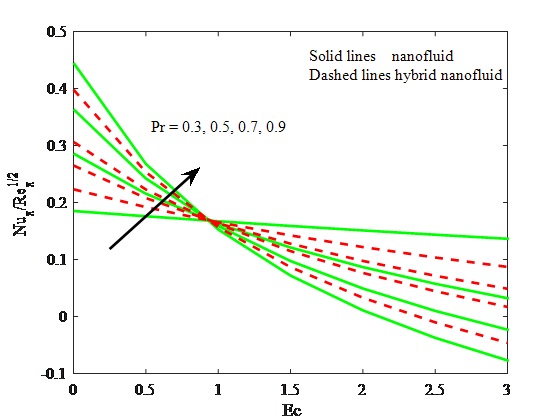
Fluctuation in skin friction coefficient is presented in Fig. 1 for distinct values of Pr and A for both nanofluid and hybrid nanofluid. Here one can see that an increment in Pr and A leads to an enhancement of the friction factor for both the nanofluid and the hybrid nanofluid. Further, the nanofluid shows overriding performance compared to the hybrid nanofluid The variations in Nu x through Pr and Ec for both nano and hybrid nanofluids are described in Fig. 2. The higher Pr scale back the Nu x but in the other hand, Nu x increases for ascending values of Ec. A comparative analysis shows that the reduction in Nu x is higher for the hybrid nanofluid case than the nanofluid. The influence of R and Pr on Nu x is portrayed in Fig. 3. This plot shows that the heat transport rate reduces for higher values of Pr, while a contradiction is recognized for increasing value of R.


The profile of θ(η) versus η is observed in Fig. 4. This figure illustrates that θ(η) is improved rapidly as R is incremented. Physically, a higher value of R corresponds to a higher thickness of the thermal layer. The larger R leads to a decrement in the coefficient of mean absorption.

Hence, the heat amount transfer to liquid is stirring. Fluctuations in θ(η) via θ w are depicted in Fig. 5. An increase in θ w corresponds to a higher temperature and thicker thermal layer. The larger θ w provides more energy to working liquid due to which presence of θ w give peak to temperature profile. Figure 6 exhibits the role of Pr on the profile of θ(η). A raise in values of Pr diminish the temperature.
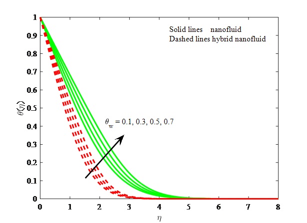

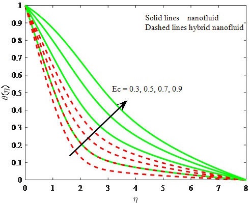
Figure 7 presents the influence of Ec on the θ(η) profile. Here, it can be noticed that the temperature and its interrelated thickness of layer is improved for increasing Ec. Basically, the existence of viscous heat in heat expressions acts as an internal heat agent. Hence, the thermal energy booming in the fluid. The effect of (2 on f(η) and θ(η) are demonstrated through Figs. 8 and 9. Figure 8 represents that for larger (2, the flow is faster for both the nanomaterial and the mixture of nanomaterials. The temperature θ(η) is found to increase for higher (2 (see Fig. 9). The nanoparticles generate warmness in liquid due to presence of photo-catalytic aspect. Hence, the addition of more nanoparticles leads to a temperature enhancement.


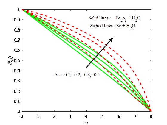
The effect of A on θ(η) is portrayed in Figs. 10 and 11. From Fig. 10, it is noticeable that the liquid is close to the surface of the solid on which the liquid flows due to a higher absolute value of A(< 0). Physically, the convection current is improved by an increase in λ. From Fig. 11, one can observe that thetemperature of the fluid scales back for larger values of A(> 0). The behavior of Φ1 on both f’(η) and θ(η) are plotted in Figs. 12 and 13. From Fig. 12, it is observed that f’(η) and its interrelated concentration layer become larger as a function of Φ1. Figure 13 indicates that the increasing behavior of θ(η) and its interrelated concentration layer is reduced due to the parameter Φ1. Figures 14 and 15 show the stream line graphs for different parameters.


Numeric values of C fx and Nu x for distinct values of influential constraints are shown in Table II. It was observed that both C fx and Nu x increase for greater values of A (see Table II).
TABLE II Numeric data of C f and Nu x corresponding to distinct values of influential constraints for both nanofluid and hybrid nanofluid.
| Pr | Ec | θw | R | A | −C fx | NU x | ||
| Hybrid nanofluid | Nanofluid | Hybrid nanofluid | Nanofluid | |||||
| 0.1 | 0.466102 | 0.463552 | 0.177526 | 0.176076 | ||||
| 0.3 | 0.462809 | 0.461259 | 0.191266 | 0.192070 | ||||
| 0.5 | 0.368881 | 0.368685 | 0.191602 | 0.208061 | ||||
| 0.1 | 0.478132 | 0.469114 | 0.252315 | 0.191266 | ||||
| 0.3 | 0.467101 | 0.465370 | 0.228968 | 0.186031 | ||||
| 0.5 | 0.464508 | 0.463552 | 0.208061 | 0.181655 | ||||
| 0.1 | 0.463940 | 0.462285 | 0.183255 | 0.180411 | ||||
| 0.2 | 0.464503 | 0.462397 | 0.186977 | 0.181097 | ||||
| 0.3 | 0.464974 | 0.462963 | 0.191973 | 0.182820 | ||||
| 0.1 | 0.466745 | 0.465113 | 0.158576 | 0.177080 | ||||
| 0.2 | 0.465981 | 0.464644 | 0.162353 | 0.179877 | ||||
| 0.3 | 0.465214 | 0.464132 | 0.166506 | 0.183226 | ||||
| 0.1 | 0.087640 | 0.089699 | 0.170182 | 0.186840 | ||||
| 0.2 | 0.061450 | 0.078860 | 0.171862 | 0.187095 | ||||
| 0.3 | 0.193750 | 0.209747 | 0.173408 | 0.193058 | ||||
Moreover Nu x rises with R and θ w . Furthermore, from Table II one can see that Nu x decreases with Ec. It can be noted from Table II that the thermal conductivity of hybrid nanomaterials high in comparison to a regular nanomaterial.
5. Conclusions
The impact of hybrid nanoparticles on fluid flow on a moving plate in the presence of thermal radiation is evaluated. The nonlinear thermal radiation is considered in the energy expression. Further, we visualized that the admixture of distinct nanomaterials corresponds to a high heat capacity in comparison to a regular nanofluid. The most notable outcomes of this study are:
The addition of hybrid nanomaterials has an positive impact on efficiency in the process of heat transport in comparison to a regular nanoparticles mixture.
The temperature field is found to decrease rapidly for distinct values of A < 0.
An increase in heat is noted for larger values of R. This translates into a temperature rise for big values of the radiation parameter.
A high Prandtl number Pr corresponds to a lower θ(η) profile. This is due to the low thermal diffusivity caused by Pr.
Temperature θ(η) increases for larger values of ϕ1.
An increment in ϕ2 resulted in an improvement in both f’(η) and θ(η) profiles.
Nomenclature
| A | velocity ratio parameter |
| Ec | Eckert number |
| T(k) | temperature of nanofluid |
| T∞ | temperature of ambient fluid |
| ρ nf (Kg m−3) | Nanofluid effective density |
| µ nf (Ns m−2) | Nanofluid effective viscosity |
| α nf (m2 s−1) | Nanofluid thermal diffusivity |
| ρ hnf (Kg m−3) | effective density of the hybrid nanofluid |
| µ hnf (Ns m−2) | effective viscosity of hybrid nanofluid |
| k nf (W K−1m−1) | effective thermal conductivity of nanofluid |
| Φ1 | solid volume-fraction of aluminium nanoparticle |
| Φ2 | solid volume-fraction of copper nanoparticle |
| ρ f (Kg m−3) | reference density of fluid fraction |
| ρ s (Kg m−3) | solid-fraction reference density |
| ρ s1 (Kg m−3) | solid-fraction reference density |
| ρ s2 (Kg m−3) | solid-fraction reference density |
| K f (W K−1m−1) | fluid thermal conductivity |
| K s (W K−1m−1) | solid thermal conductivity |
| K s1 (W K−1m−1) | solid alumina thermal conductivity |
| K s2 (W K−1m−1) | solid copper thermal conductivity |
| C s (J K−1) | heat capacity of solid surface |
| Pr | Prandtl number |
| R | radiation parameter |
| Re x | Reynolds Number |

